An Improved Algorithm for Redundancy Detection Using Global Value Numbering

Article information

Abstract

1. Introduction

Global value numbering (GVN) is a popular method for detecting equivalence among program expressions. A GVN algorithm is considered to be complete (or precise), if it can detect all of the Herbrand equivalences from amongst the program expressions. Two expressions are said to be Herbrand equivalent (or transparent equivalent) if they are computed by the same operator that has been applied to equivalent operands [1–3].

Even though GVN has many applications, as mentioned in [1], its main application is for code optimization in compilers, especially in detecting value based redundancies. The idea of using GVN for identifying value-based redundancies was conceived by Kildall [4]. In fact, Kildall formulated this with the aim of detecting common subexpressions in programs. An optimization using this algorithm will also subsume local value numbering [5, 6]. Kildall’s GVN algorithm is well known for its precision, but is not considered efficient. Most of the efficient GVN algorithms that followed Kildall concentrate on detecting equalities among variables and hence, are limited in their ability to identify value-based redundancies [3, 7]. Rosen et al. [2] is an attempt at using GVN for partial redundancy elimination (PRE) [8–10]. Briggs et al. [11] give a comparison of the different techniques for value numbering with respect to their use in different kinds of optimizations. A recent work of VanDrunen and Hosking [12] is on the use of GVN for PRE. Most of the GVN algorithms [3, 7, 13, 14] require the program to be represented in static single assignment (SSA) form [15].

Gulwani and Necula [1] (hereafter referred to as GVN-GN) is a recent polynomial time algorithm for GVN. Similar to Kildall [4], this algorithm is also based on abstract interpretation. GVN-GN is designed to detect Herbrand equivalences among terms that are of size at most s, where s is the program size. A data structure called Strong Equivalence DAG (SED) is used for representing the equivalence information at any program point. The SED is a directed acyclic graph (DAG) representation of expressions, in which the common substructures are shared. Associated with each kind of node in the flow graph, a transfer function is defined. Given an SED at the input point of a node, the algorithm computes the SED at the output point of the node by using the transfer function associated with the node. For a join node, GVN-GN uses a Join function to compute the join of the input SEDs. Given two SEDs, the Join function does a variable-based intersection of the input SED nodes. Hence, the algorithm is complete in detecting Herbrand equivalences among program variables. However, a variable based intersection limits the application of this algorithm in redundancy detection. We have observed that it is possible to miss some of the redundancies, including instances of the classical common subexpression elimination and local value numbering.

In fact, at a join point, by doing a pair of wise intersection of all the SED nodes, the algorithm could achieve completeness in detecting all Herbrand equivalences. But then, theoretically, a join of multiple SEDs can yield an exponential number of nodes in the resulting SED. The important observation is that for the purpose of redundancy detection, it is not necessary to keep all of the SED nodes that result from a join. The basic idea is to keep only those SED nodes that represent terms that are anticipable at the join point. With this, we limit the number of SED nodes to at most n_e, where n_e is the maximum number of expressions in the program.

Our algorithm requires a preprocessing stage, which will annotate every program point with the set of anticipable expressions at that program point. At the join points, GVN-GN computes a variable-based intersection of the SED nodes. With the additional step of computing a term-based intersection, we get the equivalence information that is required for identifying value-based redundancies. The result is an efficient GVN algorithm that can be directly used for identifying value-based redundancies. We show that the running time of the algorithm is a polynomial in the number of expressions in the program. Even though our emphasis is on detecting total redundancies, these improvements make the algorithm easily extendable to the general problem of detecting value-based partial redundancies.

We start with a simplified overview of GVN-GN in Section 2. We present some cases of missing equivalences in Section 3. This is followed by a presentation of our method of computing an anticipability-based join in Section 4. A proof of correctness and an analysis of the running time of the improved algorithm are given in Section 5. Some additional issues with GVN-GN are presented in Section 6, and in Section 7 we present our conclusions.

2. The GVN Algorithm by Gulwani and Necula [1]: An Overview

Gulwani and Necula [1] present a polynomial time algorithm for GVN. The algorithm is designed to detect Herbrand equivalences among terms that are of size at most s, where s is the program size. We will now present a brief overview of the algorithm. In our discussions, we follow the same notations as in [1].

2.1 Representation of Equivalence Information

A data structure called SED is used for representing the equivalence information at every program point. The SED is a directed acyclic graph representation of expressions. It is similar to the structured partition DAG in [16]. Each SED represents a partition of expressions and each node in the SED represents an equivalence class. A node is denoted by <V, t>, where V is a set of program variables labeling the node and t is the type of the node. A node with type ⊥ or c (a constant) has no successors, whereas, a node with type F(η₁, η₂) has two ordered successors, η₁ and η₂. For example, Fig. 1 shows a program node containing the assignment z := F(x, y), and two SEDs G_in, and G_out representing the equivalence information at its input and output points, respectively. Here G_in consists of three nodes and it represents the partition {[z], [x, 1], [y, 2]}. In G_out, the node <z, F> has two successors, <x, 1> and <y, 2>. This node represents the equivalence class [z, F(x, y), F(1, y), F(x, 2), F(1, 2)].

Fig. 1

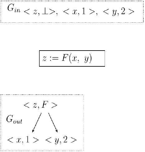
SEDs representing equivalence information.

2.3 Join Function

The equivalence information at the input of a join node is computed by means of a Join function. Given two SEDs, G₁ and G₂, and an integer s′, Join (G₁, G₂, s′) returns an SED G such that G implies all equivalences among terms that are of size at most s′, that are implied by both G₁ and G₂. The basic step in Join is the invocation of a recursive function Intersect (Node_G1(x), Node_G2(x)), for every variable x in the program (Node_Gi(x) returns the node in SED G_i, with label x). For SED nodes η₁ and η₂, Intersect (η₁, η₂) returns an SED node η such that η represents all expressions that are of size at most s′ and that are represented by both η₁ and η₂.

2.3.1 Computing Join: An Example

Fig. 2 shows a program fragment with the SEDs that GVN-GN computes at program points p₁, p₂ and p₃. G_i is the SED at program point p_i. SED G₃ results from the join of G₁ and G₂. The Join algorithm invokes Intersect() for each variable. Intersect (<x, 1>, <x, 3>) results in the node <x, ⊥> in G₃ and Intersect (<y, 2>, <y, 4>) results in the node <y, ⊥> in G₃. The node <z, F> in G₁ represents the equivalence class [z, F(x, y), F(1, y), F(x, 2), F(1, 2)]. The node <z, F> in G₂ represents the equivalence class [z, F(x, y), F(3, y), F(x, 4), F(3, 4)]. Intersect (<z, F>, <z, F>) results in the node <z, F> in G₃, which represents [z, F(x, y)].

Fig. 2

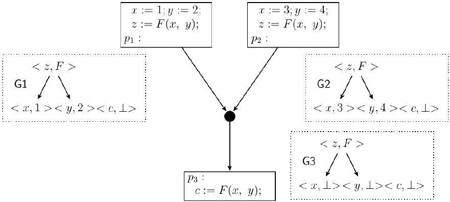
Join of SEDs: G_i is the SED at program point p_i. G₃= Join(G₁, G₂).

3. GVN-GN and Detection of Value Based Redundancies

Let us now look at how we can make use of the equivalence information computed by GVN-GN in detecting value based redundancies. Consider a node n that contains an expression e. Let G_in be the SED computed by the algorithm at the entry of n. If e ∈ Terms (η) for some node η in G_in, then we can conclude that whenever control reaches the entry of n, an expression equivalent to e has been already computed and hence, the occurrence of e in n is redundant. For example in Fig. 2, for the SED G₃, F(x, y) ∈ Terms (z, F). This indicates that when control reaches the point p₃, in every path reaching p₃, an expression equivalent to F(x, y) is computed. Hence, it is clear that the occurrence of F(x, y) in the last node is redundant.

What we have shown in Fig. 2 is an example for which the algorithm works fine. However, we have observed that there are cases for which the computed SED does not have the information required for redundancy detection, thereby limiting the use of this algorithm in related applications. In the following section, we show some examples of equivalences missed by GVN-GN.

3.1 Case of Missing Equivalences

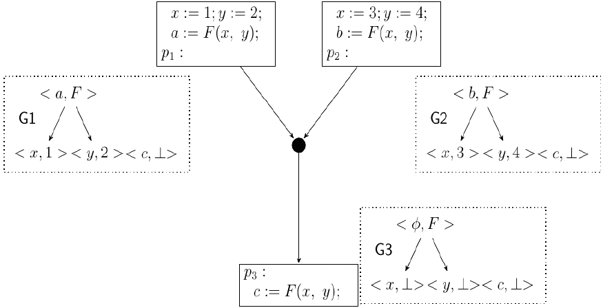
Fig. 3 shows an example which, similar to Fig. 2, is a case where the occurrence of F(x, y) in the last node is redundant. We will now show that with the equivalence information computed by GVN-GN, it is not possible to detect this redundancy. The basic step in the Join algorithm invokes Intersect ( ) for each variable. For the variable a, Intersect (<a, F>, <a, ⊥>) results in <a, ⊥> in G₃. For the variable b, Intersect (<b, ⊥>, <b, F>) results in <b, ⊥> in G₃. The case for the variables x, y and c is also similar. In G₁, F(x, y) ∈ Terms (<a, F>) and in G₂, F(x, y) ∈ Terms (<b, F>). But for no node η in G₃, F(x, y) ∈ Terms (η). As such, the redundancy in this case goes undetected. To have F(x, y) represented by a node in G₃, there should be an invocation of Intersect (<a, F>, <b, F>). However, this is never invoked from Join (G₁, G₂).

Fig. 3

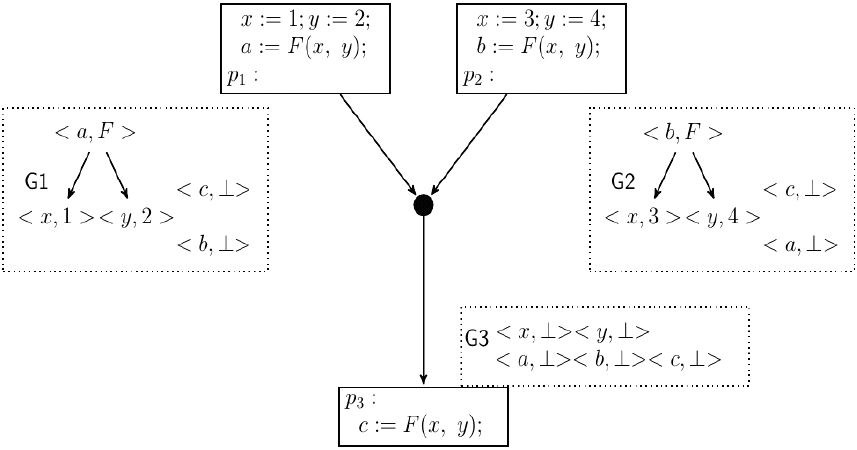
Case of missing equivalences: for program point p_i, G_i is the SED that GVN-GN computes. G₃= Join(G₁, G₂). Intersect (<a, F>,<b, F) is not invoked.

The examples in Figs. 2 and 3 are similar except in the names of variables. The reason why Gulwani and Necula [1] fails in the second example is that there are no common variables labeling the nodes representing the expression F(x, y). This will be the case with any GVN algorithm that detects variable based equalities. The example clearly shows that this is not enough for redundancy detection in general.

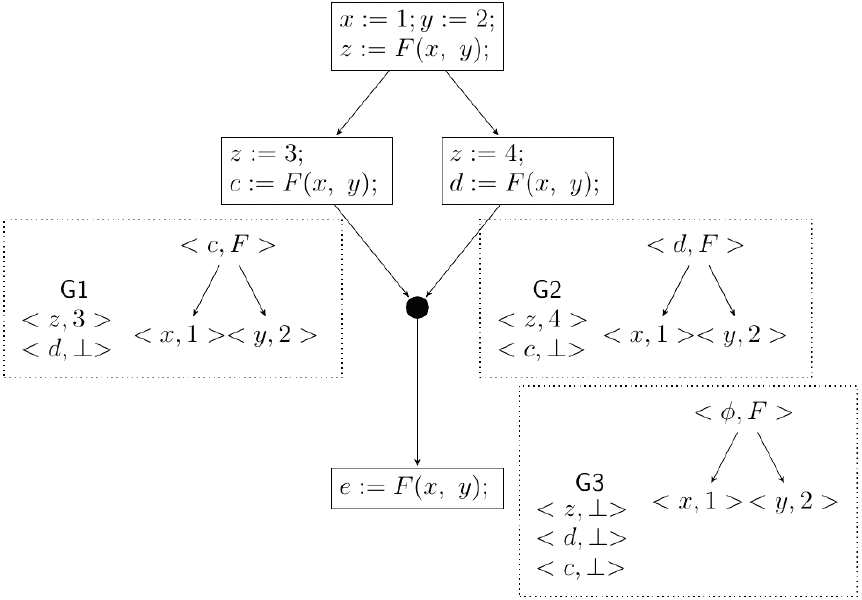
Fig. 4 shows an additional example in which all the occurrences of F(x, y) are Herbrand equivalents. The node <c, F> in G₁ represents the equivalence class [c, F(x, y), F(1, y), F(x, 2), F(1, 2)] and the node <d, F> in G₂ represents the equivalence class [d, F(x, y), F(1, y), F(x, 2), F(1, 2)]. But there is no node in G₃ that represents the equivalence class [F(x, y), F(1, y), F(x, 2), F(1, 2)]. Here, whenever control reaches p₃, an expression equivalent to F(x, y) is already computed. However, there is no way to deduce this information from the SED G₃.

Fig. 4

Case of missing equivalences: for program point p_i, G_i is the SED that GVN-GN computes. The expression F(x, y) and its equivalent expressions are not represented in the SED G₃.

4. Anticipability-Based Join

The basic problem with the Join algorithm in GVN-GN is that it computes intersection of only those SED nodes having at least one common variable (see line 3 of the Join algorithm: for each variable x ∈ T . . . Intersect (NodeG₁(x), NodeG₂(x));). For the example in Fig. 3, in G₁, F(x, y) ∈ Terms (<a, F>) and in G₂, F(x, y) ∈ Terms (<b, F>). Now, to have F(x, y) represented by a node in G₃, there should be an invocation of Intersect (<a, F>, <b, F>). In general, if there is an expression e such that e ∈ Terms (η₁) and e ∈ Terms (η₂) for some nodes η₁ of G₁ and η₂ of G₂, then to have e represented by a node in the resulting SED there should be an invocation of Intersect(η₁, η₂). This suggests that to have the required information at a join point the Join algorithm should compute the intersection of every pair of nodes of the two SEDs that have at least one common expression. Hence, a solution that will enable the algorithm to detect these kinds of equivalences is to modify the Join algorithm in such a way that it computes the intersection of every pair of nodes in the two SEDs

The approach of computing a pairwise intersection of the SED nodes will yield a precise algorithm. But theoretically, when we compute the join of n SEDs, it can result in an SED whose size is exponential in n. Furthermore, it can result in SED nodes representing non-program expressions. Here it is important to observe that for the purpose of redundancy detection, we do not need to keep all of the resulting nodes. The idea is to keep only those nodes η such that e ∈ Terms (η) for some expression e that is anticipable at the join point. This requires a preprocessing stage to compute the set of anticipable expressions at every program point.

Fig. 5 shows the SED computed by this approach for the example in Fig. 3. The intersection of <a, F> in G₁ and <b, F> in G₂ results in the node <ϕ, F> in G₃, which represents the class [F(x, y)]. It should be noted that Gulwani and Necula [1] consider nodes like <ϕ, F> with an empty set of variables to be unnecessary. But in fact, these are necessary (as will be shown later) and as such, the proposed method will retain such nodes.

Fig. 5

Anticipability-based Join: G₃ is the SED resulting from the join of G₁ and G_2. The expression F(x, y) is represented by <ϕ, F> in G_3.

Fig. 6 shows the SED computed by the proposed method for the example in Fig. 4. The intersection of <c, F> in G₁ and <d, F> in G₂ results in the node <ϕ, F> in G₃, which represents the class [F(x, y), F(x, 2), F(1, y), F(1, 2)]. Since F(x, y) is anticipable, the method retains this node.

Fig. 6

Anticipabilty-based Join: G₃ is the SED resulting from the join of G₁ and G₂.

Join-Improved (G1, G2, s′, ant_exp) =
  1     for all nodes η1 ∈ G1 and η2 ∈ G2
  2              memoize [η1, η2]:= undefined;
  3     G = ϕ_;
  4     for each variable x ∈ T in the order <G1 do
  5              counter := s′;
  6              Intersect (NodeG1(x), NodeG2(x));
  7     for each expression e ∈ ant_exp do
  8              counter := s′;
  9              Intersect (FindNode (G1, e), FindNode (G2, e));
10     return G;

FindNode (G, e) =
       1      match e with
       2 y: return NodeG(y);
       3 F(e1, e2):let η1 = FindNode(G,e1)and η2 = FindNode(G,e2)
       4             in if (<V, F (η1, η2)>) ∈ G return (<V, F (η1, η2)>);
       5                                     else return (<ϕ, ⊥ >);

5. Correctness Proof and Analysis

In this section, we present the correctness proof and time complexity analysis of the improved algorithm.

6. GVN-GN: Problems with the Removal of SED Nodes

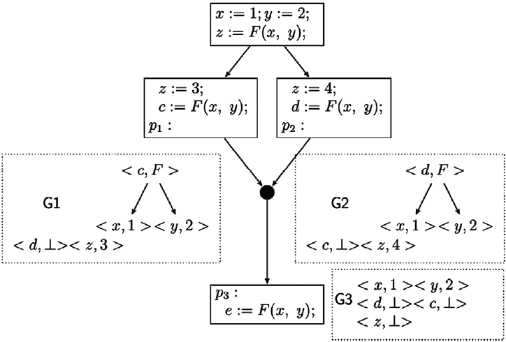
Here we will discuss an additional problem with GVN-GN that prevents the detection of some of the equivalences that even a local value numbering algorithm will detect. Fig. 7 shows a basic block in a program with the SEDs G₁ and, G₂ at program points p₁ and p₂, respectively. The expressions F(x, y) and the two occurrences of F(a, b) are equivalent and this equivalence will be detected by a local value numbering algorithm [2]. It goes undetected in Gulwani and Necula [1] because of the reasons laid out below.

Fig. 7

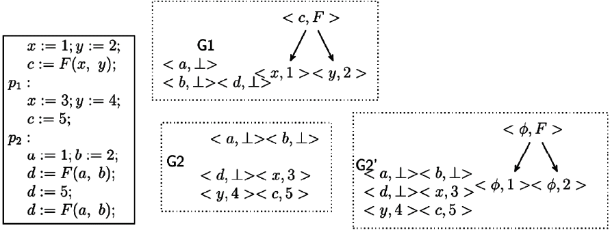
Removal of “unnessary” nodes: G₁ and G₂ are the SEDs at points p₁ and p_2, respectively. G₂′ is the SED required at p₂.

In Section 3.1 of Gulwani and Necula [1], it is stated that the transfer functions may yield SEDs with unnecessary nodes, and that these unnecessary nodes may be removed (a node is considered unnecessary when all of its ancestor nodes or all of its descendant nodes have an empty set of variables). Also, it is stated in Section 5.1 that the data structure (SED) represents only those partition classes that have at least one variable. G₂′ is the SED that would have been computed if there is no removal of SED nodes. Nevertheless, the algorithm considers the three nodes <ϕ, 1>, <ϕ, 2> and <ϕ, F> as unnecessary and hence these nodes will be removed. This results in SED G_2.

7. Conclusion

The main application of GVN is for code optimization in compilers, especially in detecting value based redundancies. The examples shown in Figs. 3 and 4 for the case of missing equivalences are instances of the classical common subexpressions. The example in Fig. 7 is an instance of local value numbering. These are enough evidence to show that the improvements are necessary for the practical adaptation of this GVN algorithm [1] in code optimizations. The suggested improvements result in a more precise and polynomial time algorithm for GVN.

Article information Continued