Mohaisen: A Review of Fixed-Complexity Vector Perturbation for MU-MIMO
Abstract
Recently, there has been an increasing demand of high data rates services, where several multiuser multiple-input multiple-output (MU-MIMO) techniques were introduced to meet these demands. Among these techniques, vector perturbation combined with linear precoding techniques, such as zero-forcing and minimum mean-square error, have been proven to be efficient in reducing the transmit power and hence, perform close to the optimum algorithm. In this paper, we review several fixed-complexity vector perturbation techniques and investigate their performance under both perfect and imperfect channel knowledge at the transmitter. Also, we investigate the combination of block diagonalization with vector perturbation outline its merits.
Key words: Block Diagonalization, MU-MIMO, Perfect and Imperfect Channel Knowledge, Quantization, Vector Perturbation
1. Introduction
Single-user multiple-input multiple-output (SU-MIMO) techniques have shown a tremendous increase in system capacity without requiring a proportional increase in the used spectrum [ 1]. In practice, a base station (BS) communicates instantaneously with several users over the same spatial-temporal resources in a scenario that is referred to as a MU-MIMO system. In comparison to SU-MIMO systems, MU-MIMO systems are shown to linearly increase the system capacity [ 2]. To match the maximum sum capacity at the downlink of the MU-MIMO system, several techniques based on dirty paper coding (DPC) have been introduced, where it has been demonstrated that the performance of the communication system with a known interference is equivalent to that of the interference-free system [ 3]. Since the BS knows the channel matrix, by means of feedback or reciprocity, and the symbols designated to all users, the inter-user interference (IUI) can be cancelled, or greatly reduced, by means of MU-MIMO precoding techniques. Linear zero-forcing (ZF) is a simple precoding technique where the direct channel inversion precoder is used at the transmitter so that each user receives its designated data with zero IUIs. When the channel matrix is ill-conditioned, the required transmit power increases to maintain a certain performance at the users’ receivers. A regularized inversion algorithm, a.k.a. minimum mean square-error (MMSE), is used where the channel matrix is regularized before inversion to avoid inverting the close-to-zero minimum singular value in the case of an ill-conditioned system. The MMSE slightly improves the performance, however, it still lacks the optimum diversity order and performance [ 4]. Lattice basis reduction techniques, such as LLL and SA, can be used to obtain a better-conditioned channel matrix, which results in better performance [ 5– 7]. Then, linear precoding techniques can be performed using the newly obtained basis of the lattice (i.e., the matrix obtained via lattice basis reduction.) These techniques achieve the optimum diversity order, whereas, to achieve the optimum performance, more powerful modifications, such as lattice-reduction with a list of candidates, can be used. The main drawbacks of the lattice basis reduction techniques are as follows: 1) they have a sequential nature that limits fast implementations via pipelining or parallelization and 2) the computational complexity (i.e., proportional to the number of iterations) depends on the conditionality of the channel matrix. As such, its worst-case value can be very high [ 8]. Tomlinson-Harashima precoding (THP) limits the transmit power by introducing the non-linear modulo operation [ 9, 10]. As a consequence, out of constellation points at the output of the precoder are rounded off to a pre-defined range. A linearized version of the THP that consists of the vector perturbation (VP) stage and IUI cancellation stage is presented in [ 11]. The VP stage disturbs the data vector such that the transmit power is reduced. Then, the same modulo operation can recover the transmitted signal at the receivers. The IUI cancellation stage can then be either done successively or by using any of the aforementioned linear precoders. Despite the improvement by THP, as compared to the linear precoders, it still lacks optimum performance and diversity order.
The VP process can be further optimized by using more efficient algorithms than the single successive interference cancellation stage employed in the THP. In this paper, we review the structure and performance of several fixed-complexity vector perturbation techniques. When the sphere encoder (SE) is used at the vector perturbation stage, it achieves the optimum performance and diversity order. However, it has a high worst-case complexity as its complexity is random and has a sequential nature that leads to high latency [ 12]. We will first introduce the QR-decomposition with the M-algorithm encoder (QRDM-E), and outline its shortages in terms of complexity and lack of pipelining capabilities [ 13]. Therefore, the fixed-complexity sphere encoder (FSE) is introduced, where both its low complexity and high parallelization capabilities are outlined [ 14]. The parallel QRDM-E (PQRDME) is then introduced, for which the goal is to reduce the computational complexity of the conventional QRDM-E [ 15, 16]. These algorithms achieve the optimum diversity order and perform close to the optimum precoder. Note that the aforementioned precoding approaches conventionally assume that a single stream transmission is employed. Block diagonalization (BD), which supports multi-stream transmission, can be used to transform the MU-MIMO channel into several parallel SU-MIMO systems that can be independently precoded [ 17– 19]. The rest of this paper is organized as follows: in Section 2 we introduce the system model and the VP. In Section 3 we formulate the VP problem and introduce conventional algorithms to solve it. In Section 4 we introduce the fixed-complexity VP algorithms. In Sections 5 and 6 we investigate the performance of the MU-MIMO system with VP and BD and with imperfect channel state information (ICSI) at the transmitter side, respectively, where simulations results are included at the end of each section. Finally, we present out conclusions in Section 7.
2. System Model and Introduction to Vector Perturbation
We implemented a downlink MU-MIMO system where a BS is equipped with nT transmit antennas and is able to instantaneously communicate with nU decentralized users that are each equipped with nR receive antennas. Without the loss of generality we assume that nT = (nU × nR), which is the minimum number of required antennas at the BS. The channel coupling transmit and receive antennas are considered to flat fading and slowly time-varying. The system is then converted to the N = (2×nT) real Euclidean system. Let H ∈ RN×N denote the channel matrix and s ∈ RN denote the data symbols, both in the real domain. Then, the precoded vector is given by:
where, γ is a scaling factor used to fix the transmit paper to a predefined value; set to unity throughout the paper. The precoding matrix P is given by H−1 and (HTH + αI)−1HT for the linear ZF and MMSE precoders, respectively. Although the MMSE precoder regularizes the channel matrix via the scalar α, the performance is still mediocre.
In order to reduce the transmit power, and instead of regularizing the channel matrix with the MMSE precoder, the VP disturbs the transmitted vector with an integer vector. This idea is based on the linearized version of the THP. The perturbed vector is given by:
where, τ is an integer given by:
with |cmax| as the absolute value of the constellation point with the largest value and Δ is the spacing between neighboring constellation points. Since the precoding ideally equalizes for the channel, the i-th received symbol is given by:
with, ni denoting the real noise at the i-th receiver with a variance of (σn2/2). The transmitted symbol is then demodulated, without knowing t, using the nonlinear modulo operation below:
where, Q(.) is the demodulation operator. The modulo operation reduces the range of the signal to [- K, K) with K as the square root of the cardinality of the modulation set and K = 2 and 4 for QPSK and 16-QAM schemes, respectively. Fig. 1 depicts the MU-MIMO system with VP, where the matrix F is a power control matrix. In the following section we assume that all users/streams have equal power; hence, F = I. To illustrate the idea behind VP, we used the following example where, for the sake of simplicity, the channel matrix and data vector are assumed to be real. Let:
where, based on ( 3) τ = 4. Let the elements of vector t be drawn from the set {0,1} leading to a set of candidates of t that are 23 = 8 in size. Again, for the sake of simplicity, we used ZF precoding, where, consequently, the transmit power is given by: where, the subscript i denotes the candidate’s index. The equation below depicts the candidates of t and the corresponding required transmit power. Note that ZF precoding without VP corresponds to setting all the elements of t to 0 (i.e., t0 in the equation below).
Note that the transmit power required in the cases of t7, t5, and t2 are lower than that in case of t0. The next challenge is to find the “best” t such that the required transmit power is reduced and the performance is improved.
3. Statement of Problem and Review of Conventional Algorithms
3.1 Statement of Problem
In power- and latency-limited communication systems, algorithms with deterministic, low latency are preferred compared to the stochastic ones that have high worst-case latency and computational complexity. The SE and lattice base reduction precoding, which are examples of stochastic algorithms, have been widely studied. In addition to the high worst-case computational complexity, SE has a sequential nature that leads to high latency. As for lattice basis reduction precoding, the number of iterations required to orthogonalize the lattice basis can be as high as theoretically infinite, depending on the conditioning of the channel matrix (i.e., lattice basis).
We are proposing several low and fixed computational complexity algorithms that aim to find the best t vector such that the total transmit power is reduced [ 14– 17]. That is: The size of the symmetric set Z from which the elements of t are drawn is decided using simulations (see figures in [ 14– 16]). To solve ( 6) successively, let the transpose of H be factorized into the product of the unitary matrix Q and upper triangular matrix R. Then the search problem in ( 6) is expanded to: where, sn and tn are the n-th elements of the vectors s and t, while the matrix L equals (R−1)T. In the case of MMSE precoding, the extended matrix
[HT αI]T is factorized, with α as the regularization coefficient.
3.2 Statement of Problem
The conventional THP scheme is nonlinear, due to the nonlinear modulo operation that is performed to limit the range of the precoded signal at the transmitter side. A linearized version of this scheme has been proposed in [ 11]. In correlation to the QRD-based successive interference cancellation, the THP successively searches the elements of the vector t. At each search level, the single candidate of t, which reduces the accumulative metric in ( 7) is retained. The main drawback of this method is that the elements of t are obtained independently, which leads to degradation in the system’s overall performance, in terms of BER and diversity order. Instead of retaining a single candidate at each search level, the QRDM-E retains a fixed number of candidates at each encoding level, denoted by M. Fig. 2 shows an example of the QRDM-E with an equal Z and M of 4. At the first VP level, the root node is extended to the four possible branches, where each branch represents a hypothesis of t1. Since, M = T, all the candidates are retained for the next level. All the retained candidates at the first level are extended, leading to a set of 16 hypotheses for t2. The metrics are computed based on ( 7) and sorted where the best M = 4 candidates with the least accumulative metrics are retained for the next level. This strategy is repeated until the last VP level, where the vector with the least accumulative metric is precoded and transmitted. It has been shown that the QRDM-E algorithm with sufficient M achieves quasi-optimum performance and optimum diversity order [ 13]. The main drawbacks of the QRDM-E are as follows: 1) it has a sequential nature, which limits the parallelization of the VP stage leading to high latency and 2) the computational complexity is high for a large problem size. In the next section, several algorithms are proposed in order to reduce the computational complexity, quantified in terms of the number of visited nodes in the search tree, and the latency, which is quantified by the parallelization capability of the proposed algorithms.
4. Fixed-Complexity Vector Perturbation Techniques
4.1 Parallel QRDM Encoder
Based on the conventional QRDM-E, the goal of the PQRDME is to achieve a tradeoff between system performance and encoding throughput (i.e., VP speed). To achieve that, we followed the steps laid out below.
The set of candidates for the elements of the vector t is divided into G non-overlapping subsets, U1, U2, …, UG of equal sizes.
-
The VP tree-search of the conventional QRDME is then divided into G independent partial VPs (PVPs) that are pipelined, where:
In the i-th PVP, the candidates for t1 are drawn from the subset Ui. The candidates for the remaining elements of t are drawn from the full set Z. All the candidates of t are retained at the first p encoding levels. For example, in PQRD-ME-p1 and PQRDME-p2 all candidates are retained up to the first and to the second VP levels, respectively. At the remaining levels, p+1 … N, M/G candidates are retained at each encoding level per PVP leading to a total of M retained candidates per encoding level.
The vector with the least accumulative metric is retained at each PVP. These vectors are compared in terms of their accumulative metrics, where the one with the least accumulative metric and the one with the least global accumulative metric is encoded and transmitted.
Fig. 3 depicts an example of the PQRDME for T = 4, G = 2, M = N = 4 and p = 1. As such, at the first VP level, the set of four elements of Z is divided into the subsets U 1 and U 2, which each contain two elements. The candidates for t1 in the first PVP are drawn from U 1, whereas, the candidates for t1 in the second PVP are drawn from U 2. At the first VP level, all candidates are retained. In each PVP, the candidates for t2 to t4 are drawn from the full set Z, where at each level only M/G = 2 candidates with the least accumulative metrics are retained. The process is repeated up to the last VP level where the vector with the least accumulative metric is selected, precoded, and transmitted.
Fig. 4 depicts an example of the PQRDME for M = N = 4 and T = G = p = 2. Apart from the size of the set of hypothesis Z, the difference with the preceding example is that all candidates are retained at both the first and second VP levels. It worth remembering that the candidates of t2, …, t4 are drawn from the full set Z.
4.2 Fixed-Complexity Sphere Encoder
The FSE has two goals: 1) increasing the encoding throughput by fully pipelining the VP stage and 2) decreasing the complexity via performing fewer computations in terms of the number of visited nodes and total number of comparisons.
To this end, the FSE consists of the following two stages:
Full expansion: At the first p tree search levels, the retained branches are expanded to all possible nodes, and all the resulting branches are retained for the next level. Single expansion: Only a single expansion is performed from each retained node at the precedent encoding level. This is done by following the decision-feedback equalization path.
At the last VP level, the accumulative metrics of the obtained vectors are compared and the one with the smallest accumulative metric is selected, precoded, and transmitted. It has been shown in [ 14] that the complexity of the FSE is about 15% of that of the conventional QRDME for T = 7, whereas, the encoding throughput is increased seven-fold.
Fig. 5 depicts an example of the FSE for T = N = M = 4 and p = 1. In the first full expansion encoding level, all the candidates are retained for the second level. In the single expansion VP levels, all retained nodes are expanded to all possible candidates. Then, the candidate with the smallest metric is retained as in the case of a successive interference cancellation detector. In the last VP level, the vector with the least accumulative metric is selected, precoded, and transmitted. Due to this tree-search structure of the FSE, it can be pipelined. This results in a tremendous increase in the encoding throughput.
Fig. 6 depicts an example of the FSE with T = 3, N = 4, M = 9 and p = 2. Up to the second VP level, all candidates are retained, whereas, a single expansion is employed at the remaining VP levels.
4.3 Simulation Results
In this section, the channel state information (CSI) is considered to be perfectly known at the transmitter side. QPSK modulation is employed and the users are considered to be decentralized where each one is equipped with a single receive antenna.
Fig. 7 depicts the performance of the fixed complexity VP encoders with the quasi-optimal QRDM-E and the linear MMSE encoder. The set size, T, is set based on extensive simulations. In the case of THP no further improvement is achieved for T > 5. The performance of the PQRDME- p1, is close to that of the quasi-optimal QRDM-E while the encoding throughput is increased by a factor of G = 2. To achieve more encoding speed, the three-search can be split into four PVPs, whereas, it is clearly seen in the figure that the performance is degraded, but the maximum diversity order is still achieved. In terms of BER performance, FSE- p1 comes last with little degraded performance, while achieving the maximum encoding throughput speed.
Fig. 8 depicts the performance of the VP algorithms for p = 2 and G = 3 in the case of the PQRDME- p2. The performance of the PQRDME- p2 is closest to the QRDM-E, followed by the FSE- p2. Note that in this scenario, the PQRDME search tree consists of the three PVPs, which leads to high parallelization capability. The THP and linear MMSE encoders achieve much worse BER performance and similar diversity order of unity.
5. Vector Perturbation with Block Diagonalization
5.1 Block Diagonalization
The IUI can be fully canceled out using the BD algorithm. Therefore, BD transforms the MU-MIMO channel into parallel SU-MIMO channels. As a result, this allows for multi-stream transmission with users equipped with either the same or a different number of receive antennas. The inter-symbol interference (ISI) among symbols belonging to a certain user can be either removed at the transmitter by means of precoding, or at the receiver by employing spatial demultiplexing (i.e., detection). To reduce the complexity of the users’ receivers, we took into consideration that the channel effect is equalized for at the transmitter side by means of precoding. Moreover, we employed the already explained VP techniques [ 16, 17]. The goal of the BD is to find the matrix B such that:
where, Hi is the channel coupling of the BS transmit antennas and the receive antennas of the i-th user. 0n is an n×n zero matrix with all elements set to 0. Heff, i is the effective channel of the i-th user after block diagonalization. The matrix B is obtained using a series of singular value decompositions. Based on the second matrix of ( 9), users’ data is precoded independently. This leads to the additional parallelization of the VP stage and as a result, improves encoding throughput. In this scenario, VP techniques with random computational complexity generally require different time durations to encode each user’s data. Since all users’ data should be transmitted at the same instant, the encoding stage requires a time duration equivalent to the worst-case delay among the users. On the other hand, fixed-complexity VP algorithms require a fixed encoding duration. That is why they are preferable in such scenarios, in addition to their advantages that we have already discussed in Section 4.
5.2 Simulation Results
Fig. 9 depicts the performance of the FSE encoder as having been implemented with the BD scheme. We evaluated the system under the ( nT, nU, nR) scenario, where the BS is equipped with nT antennas and nU users that are each equipped with nR antennas. Since the attained diversity order equals min( nT, nR) = nR, as the number of users increases, the diversity order is decreased since part of the degrees of freedom are used in the IUI cancellation. It is worth mentioning that QRDM-E outperforms FSE- p2, whereas, FSE- p2 outperforms FSE- p1 in all of the simulated SNR range. The performance of all algorithms coincide when each user is equipped with a single receive antenna. This is reasonable since the diversity order achieved by all algorithms is equal to 1. As such, these algorithms can’t exploit further performance improvement or diversity order.
Fig. 10 depicts the performance of the PQRDME encoder that has been implemented with the BD. The performance gap between the QRDM-E and the PQRDME- p2 is negligible for all of the scenarios.
6. Vector Perturbation with Imperfect Channel Knowledge
6.1 Quantization Schemes
Up until this point, the CSI is considered to be perfectly known at the transmitter. In some situations, this assumption is strong and could not be considered achievable. As such, the users need to estimate, quantize, and provide a feedback of the channel coupling their receive antennas with the BS’s transmit antennas. This process, especially quantization, leads to errors in the channel and to a degradation in the achieved performance of the whole system. In the sequel, we explain two types of quantization, which are as listed below.
Lloyd-Max Quantization: Uniform quantization divides the range to which the variable belongs into equal intervals. If the variable to be quantized belongs to a certain interval, then the centroid of the interval is considered to be the quantized value. This quantizer is suitable for uniformly distributed variables, which is not the case for MIMO channels. Therefore, the non-uniform Lloyd-Max quantizer, which takes the probability density function (pdf) of the variables to be quantized into consideration, is more suitable [20–22]. The Lloyd-Max quantizer iteratively finds the intervals’ endpoints so that the mean square error between each channel coefficient and its quantized version is minimized. This can be achieved by allocating shorter intervals when the pdf has high values (i.e., the variable is the most probable) and longer intervals when the pdf has low values. Uniform Quantization: In communication systems (WiMAX, LTE/LTE-A, etc.) the channel amplitude is usually quantized and fed back to the BS in order to be used in several schemes, such as scheduling or adaptive modulation and coding. As such, it is more effective to quantize the phase of the channel coefficient as additional feedback. It is known that the phase of the channel coefficient is uniform and, hence, can be uniformly quantized.
In the following subsection, we evaluate the performance of the PQRDME-p2 under the ICSI knowledge at the transmitter as an example of the fixed-complexity VP techniques.
6.2 Simulation Results
Fig. 11 depicts the performance of the PQRDME- p2 as an example of the VP algorithms for several values of B and the number of quantization bits for the real and imaginary parts of the channel coefficient. For a low B, the BER increases, where, when B = 5 the degradation is tolerable due to the quantization error.
Fig. 12 shows the BER performance of the PQRDME- p2 for several values of B and the number of quantization bits for each phase value. B = 6 is suitable for quantizing the phase of the channel coefficients, since the degradation due to the quantization error is tolerable.
7. Conclusions
In this paper, we introduced the idea of MU-MIMO precoding with VP, where the aim of the VP stage is to reduce the transmit power and to improve the system performance via perturbing the transmit vector in such a way that the required transmit power is reduced. Since communication systems are power- and latency-limited, both low-complexity and fixed, low latencies are required for the VP techniques. Apart from the SE and the lattice-basis reduction precoding, which have high worst-case complexity and delay, we introduced two main fixed complexity VP schemes—PQRDME and FSE—and two varieties of each one. We outlined the benefit of these algorithms in rendering the tree-search stage into a parallelized stage that speeds up the VP process. Furthermore, we examined the performance of these schemes under ICSI and perfect CSI knowledge at the transmitter and discussed the Lloyd-Max quantizer and uniform quantization. Finally, we investigated the combination of the VP schemes with BD where multi-stream transmission becomes possible.
Biography
He received his M.S. degree in communications and signal processing from the University of Nice-Sophia Antiplois, France, in 2005 and Ph.D. from Inha University, Korea, in 2010, both in communications engineering. From 2001 to 2004, he was with the Palestinian Telecom. Co., where he was a cell planning engineer. Since Sept. 2010, he is with the Department of EEC Engineering, KoreaTech, Korea, where he is an assistant professor. His research interests include 3GPP LTE/-A systems, MIMO detection and precoding and social networks.
References
1. IE. Telatar, "Capacity of multi-antenna Gaussian channels," European Transactions on Telecommunications, vol. 10, no. 6, pp. 585-595, 1999.  2. W. Yu, and J. Cioffi, "Sum capacity of Gaussian vector broadcast channels," IEEE Transactions on Information Theory, vol. 50, no. 9, pp. 1875-1892, 2004. 3. M. Costa, "Writing on dirty paper," IEEE Transactions on Information Theory, vol. 29, no. 3, pp. 439-441, 1983. 4. CB. Peel, BM. Hochwald, and AL. Swindlehurst, "A vector-perturbation technique for near-capacity multiantenna multiuser communication. Part I: Channel inversion and regularization," IEEE Transactions on Communications, vol. 53, no. 1, pp. 195-202, 2005. 5. AK. Lenstra, HW. Lenstra, and L. Lovasz, "Factoring polynomials with rational coefficients," Mathematische Annalen, vol. 261, no. 4, pp. 515-534, 1982. 6. C. Windpassinger, and RFH. Fischer, "Low complexity near-maximum-likelihood detection and precoding for MIMO systems using lattice reduction," in Proceedings of 2003 IEEE Information Theory Workshop, Paris, France, 2003, pp. 345-348. 7. M. Seysen, "Simultaneous reduction of a lattice basis and its reciprocal basis," Combinatorica, vol. 13, no. 3, pp. 363-376, 1993. 8. J. Jalden, D. Seethaler, and G. Matz, "Worst- and average-case complexity of LLL lattice reduction in MIMO wireless systems," in Proceedings of IEEE International Conference on Acoustics, Speech and Signal Processing (ICASSP2008), Las Vegas, NV, 2008, pp. 2685-2688. 9. M. Tomlinson, "New automatic equalizer employing modulo arithmetic," Electronics Letters, vol. 7, no. 5, pp. 138-139, 1971. 10. H. Harashima, and H. Miyakawa, "Matched-transmission technique for channels with intersymbol interference," IEEE Transactions on Communications, vol. 20, no. 4, pp. 774-780, 1972. 11. J. Liu, and W. Kizymien, "Improved Tomlinson-Harashima precoding for the downlink for multi-user MIMO systems," Canadian Journal of Electrical and Computer Engineering, vol. 32, no. 3, pp. 133-144, 2007. 12. BM. Hochwald, C. Peel, and AL. Swindlehurst, "A vector-perturbation technique for near-capacity multiantenna multiuser communication. Part II: Perturbation," IEEE Transactions on Communications, vol. 53, no. 3, pp. 537-544, 2005. 13. J. Zhang, and KJ. Kim, "Near-capacity MIMO multiuser precoding with QRD-M algorithm," in Proceedings of 39th Asilomar Conference on Signals, Systems and Computers (ACSSC), Pacific Grove, CA, 2005, pp. 1498-1502.
14. M. Mohaisen, and K. Chang, "Fixed-complexity sphere encoder for multi-user MIMO systems," Journal of Communications and Networks, vol. 13, no. 1, pp. 63-69, 2011. 15. M. Mohaisen, A. Mohaisen, Y. Li, and P. Luo, "Parallel QRD-M encoder decentralized for multi-user MIMO systems," in Proceedings of 2011 IEEE International Conference on Communications (ICC), Kyoto, Japan, 2011, pp. 1-5. 16. M. Mohaisen, A. Mohaisen, and M. Debbah, "Parallel QRD-M encoder for multi-user MIMO systems," Telecommunication Systems, vol. 57, no. 3, pp. 261-270, 2014. 17. M. Mohaisen, B. Hui, K. Chang, S. Ji, and J. Joung, "Fixed-complexity vector perturbation with block diagonalization for MU-MIMO systems," in Proceedings of 2009 IEEE 9th Malaysia International Conference on Communications (MICC), Kuala Lumpur, Malaysia, 2009, pp. 238-243. 18. K. Zu, RC. de Lamare, and M. Haardt, "Generalized design of low-complexity block diagonalization type precoding algorithms for multiuser MIMO systems," IEEE Transactions on Communications, vol. 61, no. 10, pp. 4232-4242, 2013. 19. L. Liang, W. Xu, and X. Dong, "Limited feedback-based multi-antenna relay broadcast channels with block diagonalization," IEEE Transactions on Wireless Communications, vol. 12, no. 8, pp. 2092-2101, 2013. 20. SP. Lloyd, "Least squares quantization in PCM," IEEE Transactions on Information Theory, vol. 28, no. 2, pp. 129-137, 1982. 21. J. Max, "Quantizing for minimum distortion," IEEE Transactions on Information Theory, vol. 6, no. l, pp. 7-12, 1960. 22. M. Mohaisen, "Transmit antenna selection for multi-user MIMO precoding systems with limited feedback," International Journal of KIMICS, vol. 9, no. 2, pp. 193-196, 2011.
Fig. 1
Multiuser multiple-input multiple-output (MU-MIMO) system with vector perturbation. 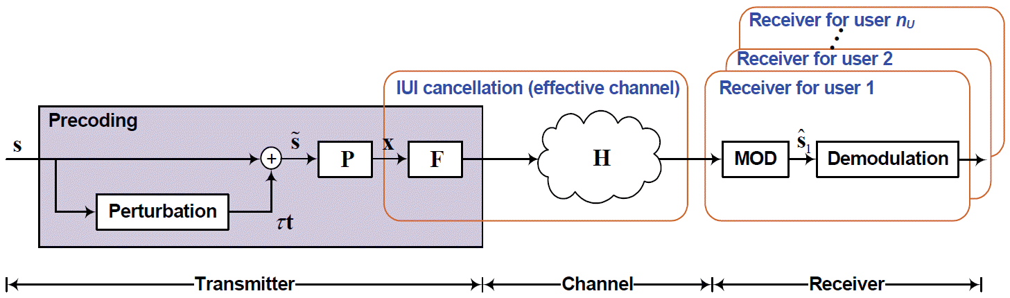
Fig. 2
An example of the QR-decomposition with the M-algorithm encoder (QRDM-E) with N = T = M = 4. 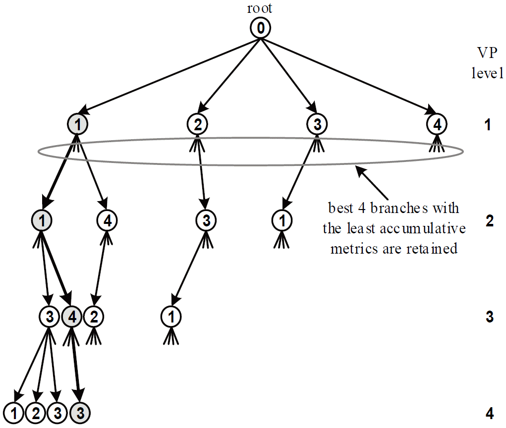
Fig. 3
An example of the parallel QR-decomposition with the M-algorithm encoder (PQRDME) for T = M = N = 4, G = 2 and p = 1. 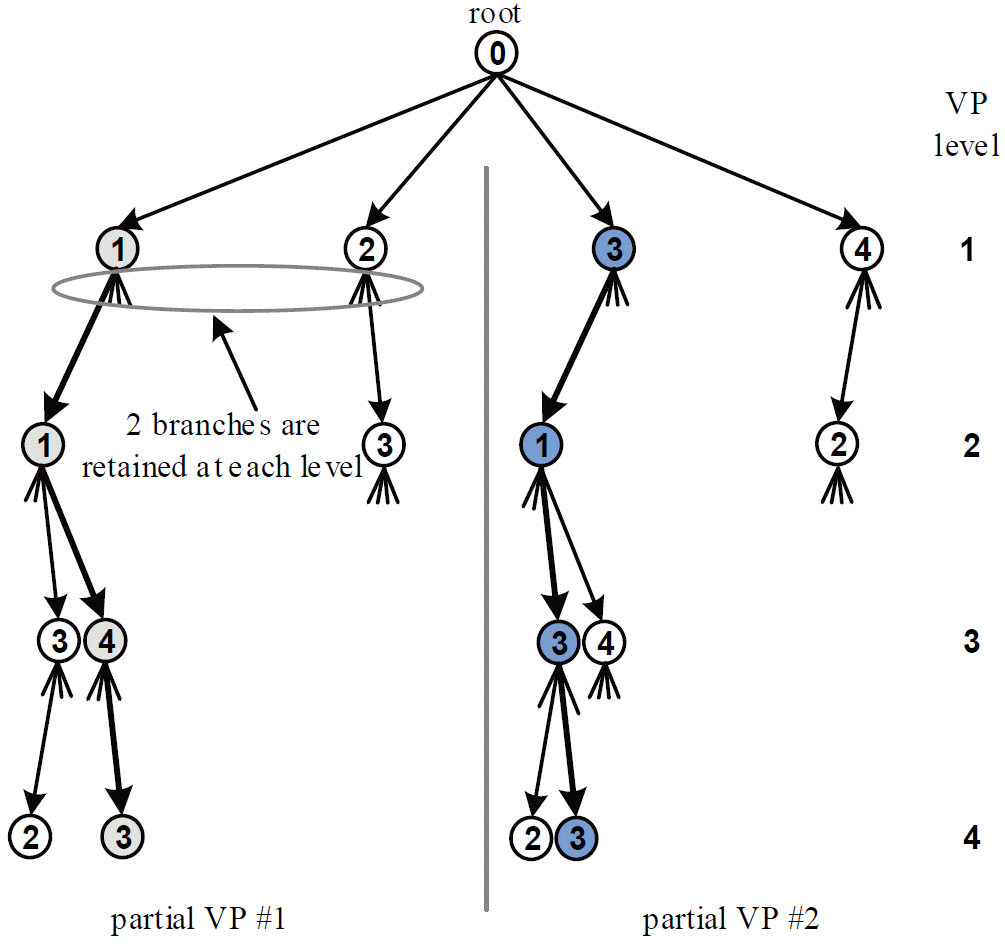
Fig. 4
An example of the parallel QR-decomposition with the M-algorithm encoder (PQRDME) for M = N = 4 and T = G = p = 2. 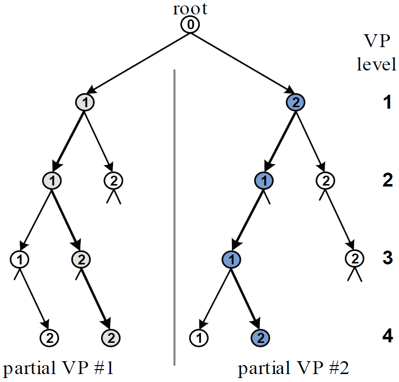
Fig. 5
An example of the fixed-complexity sphere encoder (FSE) with T = N = M = 4 and p = 1. 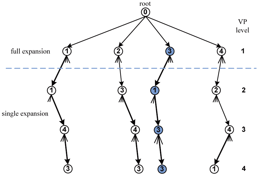
Fig. 6
An example of the fixed-complexity sphere encoder (FSE) with T = 3, N = 4, M = 9 and p = 2. 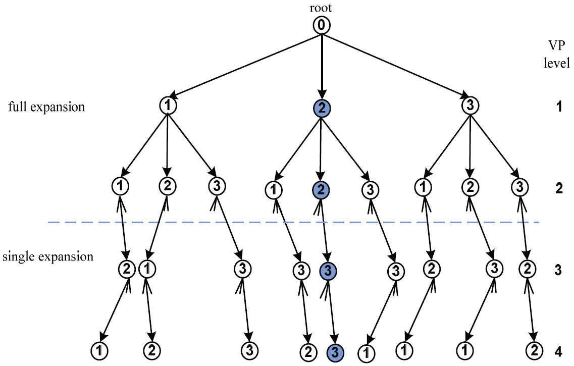
Fig. 7
Bit error rate (BER) of the fixed complexity vector perturbation schemes for a p = 1. SNR=signal-to-noise ratio, MMSE=minimum mean square error, THP=Tomlinson-Harashima precoding, FSE=fixed-complexity sphere encoder, QRDME=QR-decomposition with the M-algorithm encoder, PQRDME= parallel QRDME. 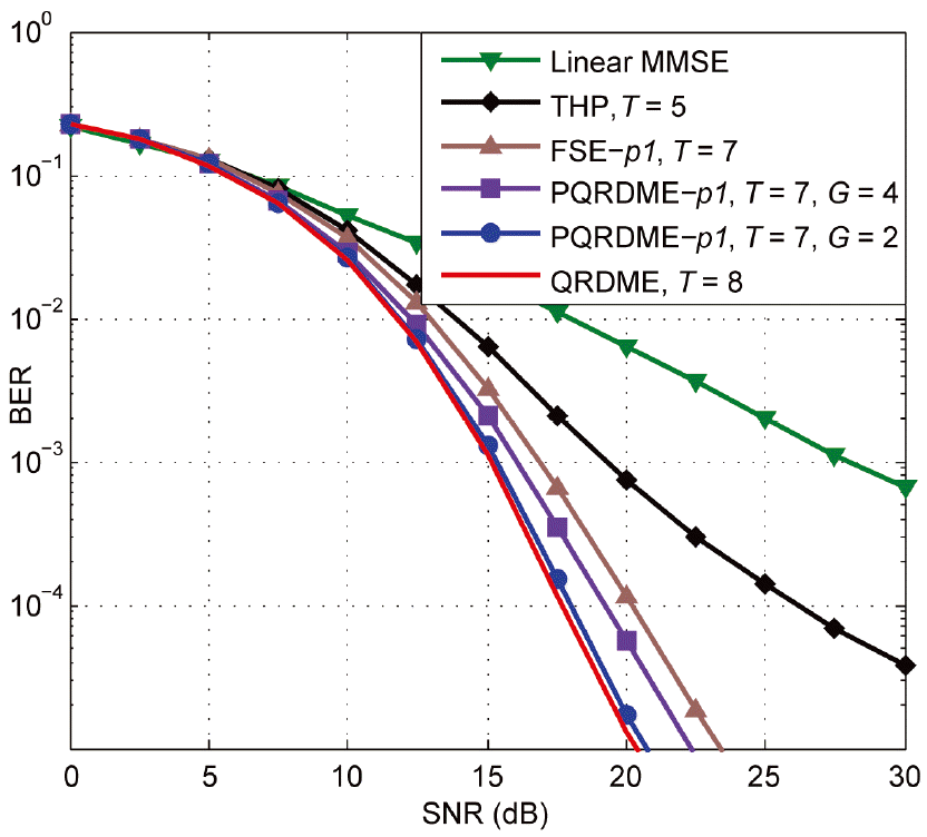
Fig. 8
Bit error rate (BER) of the fixed complexity vector perturbation schemes for a p = 2. SNR=signal-to-noise ratio, MMSE=minimum mean square error, THP=Tomlinson-Harashima precoding, FSE=fixed-complexity sphere encoder, QRDME=QR-decomposition with the M-algorithm encoder, PQRD-ME=parallel QRDME. 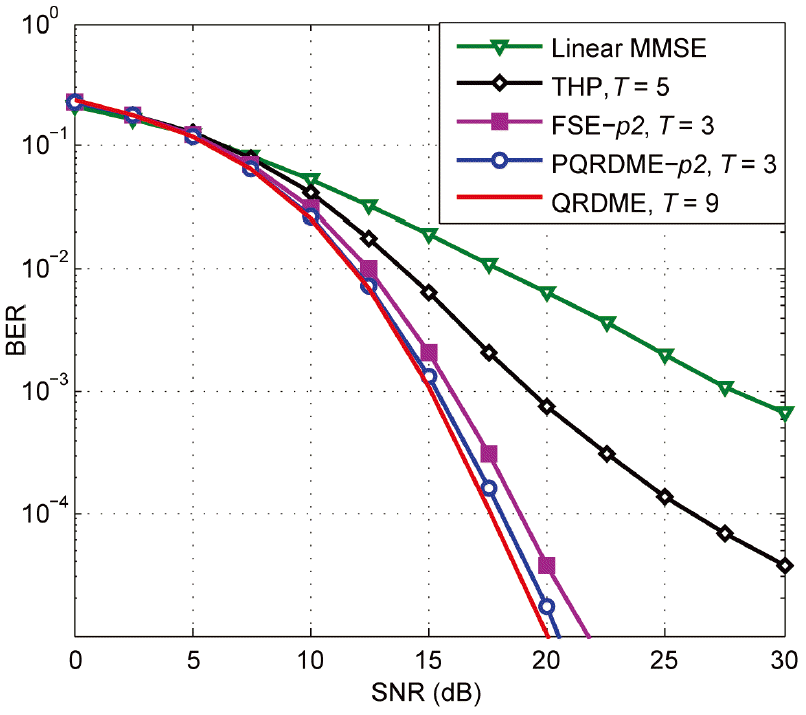
Fig. 9
Bit error rate (BER) performance of the FSE-p1 and FSE-p2 for T = 3 and T = 7, respectively, with block diagonalization. SNR=signal-to-noise ratio, FSE=fixed-complexity sphere encoder, QRD-ME=QR-decomposition with the M-algorithm encoder. 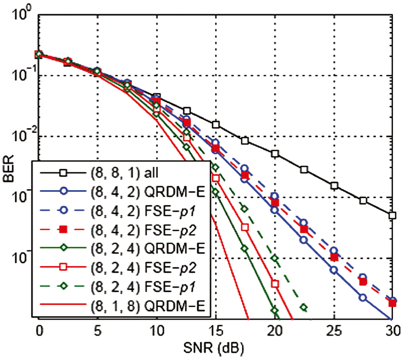
Fig. 10
Bit error rate (BER) performance of the PQRDME-p2 for T = 3 with block diagonalization. SNR=signal-to-noise ratio, QRDME=QR-decomposition with the M-algorithm encoder, PQRDME= parallel QRDME. 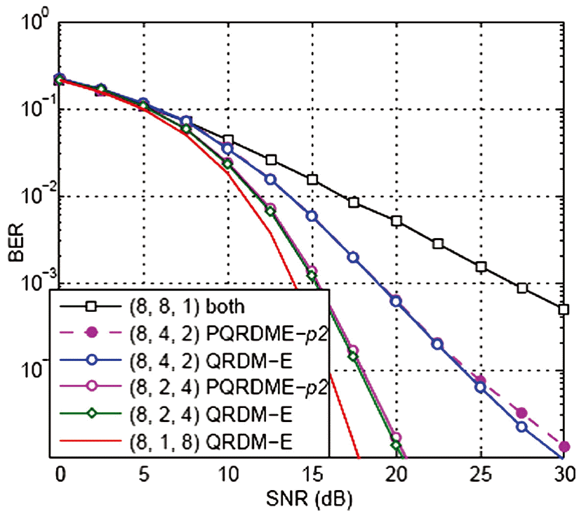
Fig. 11
Bit error rate (BER) of the PQRDME-p2 for G = T = 3 and N = 8 under imperfect channel state information with Lloyd-Max quantization. SNR=signal-to-noise ratio, QRDME=QR-decomposition with the M-algorithm encoder, PQRDME=parallel QRDME. 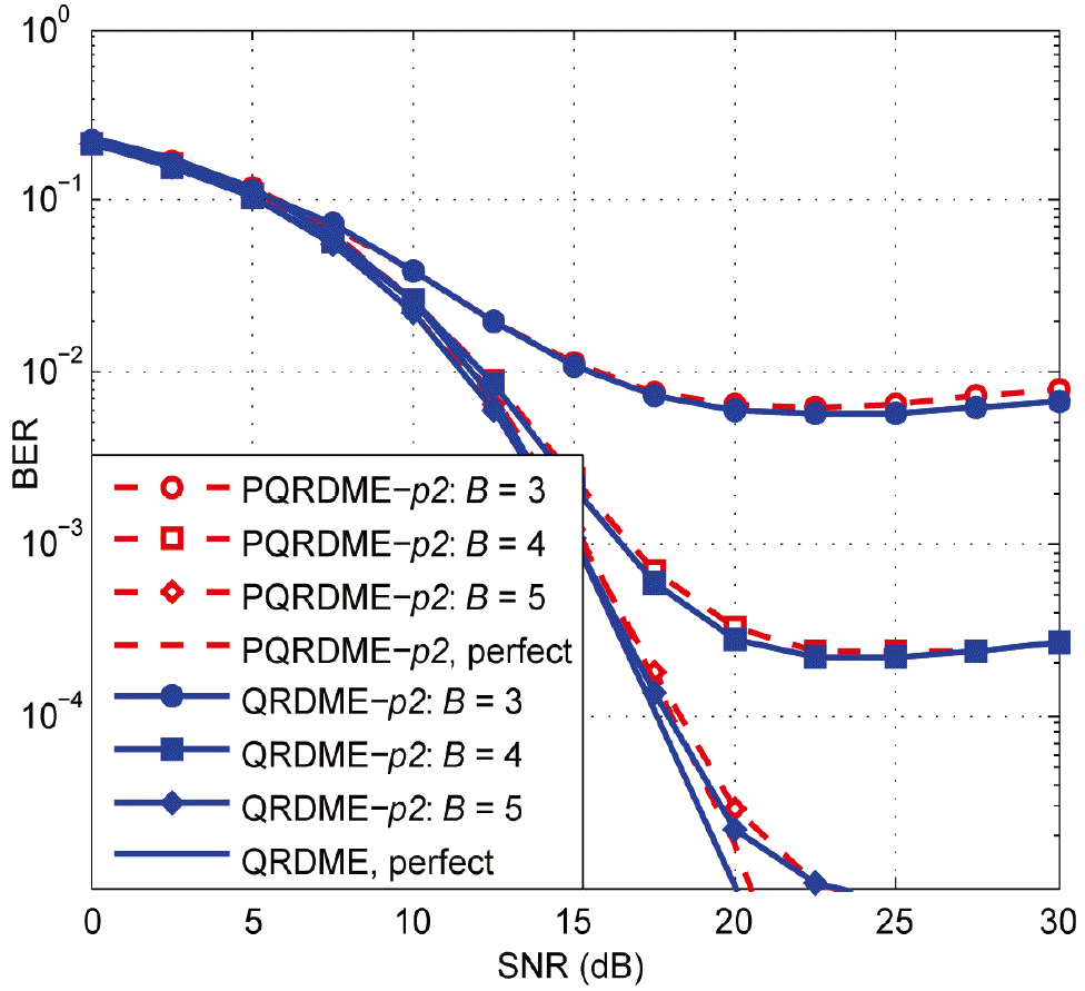
Fig. 12
Bit error rate (BER) of the PQRDME-p2 for G = T = 3 and N = 8 under imperfect channel state information with uniform quantization of the phase of the channel coefficients. SNR=signal-to-noise ratio, PQRDME=parallel QR-decomposition with the M-algorithm encoder. 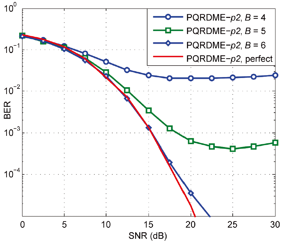
|