Nguyen and Lee: A Lightweight and Effective Music Score Recognition on Mobile Phones
Abstract
Recognition systems for scanned or printed music scores that have been implemented on personal computers have received attention from numerous scientists and have achieved significant results over many years. A modern trend with music scores being captured and played directly on mobile devices has become more interesting to researchers. The limitation of resources and the effects of illumination, distortion, and inclination on input images are still challenges to these recognition systems. In this paper, we introduce a novel approach for recognizing music scores captured by mobile cameras. To reduce the complexity, as well as the computational time of the system, we grouped all of the symbols extracted from music scores into ten main classes. We then applied each major class to SVM to classify the musical symbols separately. The experimental results showed that our proposed method could be applied to real time applications and that its performance is competitive with other methods.
Key words: Mobile Camera, Music Score, SVM, Symbol Classification
1. Introduction
Nowadays, the explosion of mobility is setting a new standard for the information technology industry. Mobile devices are not limited to calling or texting. They cover a variety of entertainment arenas, such as multimedia applications. One of the entertainment applications, which has potential and is interesting, is playing music scores captured directly from a mobile camera. In the early stages, systems for recognizing and playing OMR-based music scores on standalone PCs have been introduced [ 1– 7]. However, such systems are relatively heavy because of having to adopt machine learning algorithms [ 8– 12]. These could be difficult to deploy on mobile devices with limited computational resources. Moreover, they only work well with music scores that are captured from scanners in terms of guaranteeing the quality of the input data [ 8, 9]. Meanwhile, music scores captured directly from the mobile camera could be affected by illumination, distortion, and different viewpoints (as shown in Fig. 1). Recently, music score recognition systems have been proposed for mobile phones and have achieved potential results [ 13, 14]. These systems could overcome some problems related to illumination. But as in PC-based approaches, they still use machine learning to recognize all symbols. This is known as a relatively heavy approach to recognize musical symbols. This may lead to there being an increase in resource consumption and processing time on mobile devices. In this paper, we introduce a novel and effective approach to recognize music scores on mobile devices. First, our method deals with music scores captured directly from a mobile camera under the influences of environment acquisition, including distortion, illumination, and different viewpoints. Unlike previous approaches, our system uses some preprocessing techniques, such as global and local based binarization and the line fitting method [ 17] to eliminate the effects of the environment on input images. Moreover, to reduce the complexity, all of the symbols are grouped into 10 main classes that have the similar features before SVM is applied to recognize each symbol in these main classes. In summary, our contributions are as follows:
Our approach applies global and local threshold based binarization and the line fitting method to remove the illumination effect, distortion, and noise from input music scores to improve the performance of the system. Heuristic characteristics are used to classify all of the symbols into 10 subclasses with the similar features reduced the number of classes and the difficulty level for SVMs.
The rest of paper is organized as follows: in Section 2, we present all related works that are about recognizing the music score recognition systems. Section 3 describes the proposed method in detail. The experimental results are presented in Section 4. Finally, the conclusion and future research work are given in Section 5.
2. Related Work
Most approaches to music symbol recognition is that all symbols are split by staffs and the elementary graphic symbols such as the note head, rest, dot, stem, and tag [ 2, 6, 10, 11, 15]. Machine learning is used to recognize them. In [ 4], the k-nearest neighbor rule is used, while in [ 1, 11, 16] neural networks are the selected classifier. Choudhury et al. [ 1] proposed the extraction of symbol features, such as width, height, area, number of holes, and low-order central moments; whereas, Taubman [ 6] preferred to extract standard moments, centralized moments, normalized moments, and Hu moments with the k-nearest neighbor method. In [ 3, 12], the authors introduced various approaches that avoid the prior segmentation phase. They are superior in that, both the segmentation and recognition steps are implemented simultaneously using hidden Markov models (HMMs). Features are extracted directly from images, but this process is not only difficult to be carried out, it is also sensitive to errors. Homcnda and Luckner [ 4] used five classes of music symbols with the following two different classification approaches: classification with and without rejection. In case of leaving staff line and segmentation, [ 17] adds horizontal lines to extend to the top and bottom of the staves. [ 13, 14] are approaches for mobile devices. [ 13] applied on the Android platform and [ 14] on Windows Phone 7. Both of these methods used learning machine to recognize musical symbols from printed or camera captured music sheets
3. Proposed Method
Our proposed method provides a novel way to recognize musical symbols in music scores captured by camera. Unlike previous methods, we used two steps for recognition. In the first step, all of the symbols are classified into 10 main classes with the similarity features (number of note heads, number of lines). Each of the 10 main classes includes some of the symbol subclasses. After that, we applied the SVM method to classify separate symbols in each class.
3.1 The Overall Method
Fig. 2 presents the overall model of our proposed method. With each symbol, it would first be classified into one of 10 major classes based on heuristic criterions such as found location symbols, the number of note heads, and the number of vertical lines. These features are achieved with high accuracy by using the symbol’s proper information, projection, template matching, and shift. Each main class contains one symbol or some kind of symbol. With the later cases, nine SVMs were used to classify symbols into subclasses.
3.2 Preprocessing
This step implements two tasks, including image binarization and staff line information extraction. Under the effect of illumination, the background color of music image becomes swarthy in some cases. It is difficult to separate the background from the foreground using only the local or global threshold methods [ 17]. Therefore, the combination of the local and global threshold is used to binary image. As mentioned before, the music sheets captured on a mobile camera are often affected by distortion, illumination, and different viewpoints. Therefore, the staff lines in the achieved binary image could be distorted and tilted. To resolve this issue, we used the line fitting method [ 17] to detect and correct these staff lines.
3.3 Ten Main Classes
To achieve 10 classes from all if the symbols after segmentation, we base on the features of symbols. The 10 classes are as follows: CLEF, _NORMAL_NOTE, _BEAM_NOTE, _FULL2_NOTE, _SHARP_ NATURAL, _NO_LINE, _MULTI_NOTE, _MULTI_BEAM_NOTE, _MEASURE, and _CODE, which are shown in Table 1. With general ideal, there are three special kinds of symbols: _CLEF, _MEASURE, and _CODE. These independent on the number of note heads and number of lines and they have fixed locations on the music score. After segmentation, with the information about the locations of these symbols, we can be easy to classify them into the following three main classes: the first class is _CLEF, where the size of this symbol is large, the top and bottom boundary of the cleft are outside the top and bottom of the staff line and this symbol is located at the beginning of the stave. The second class is _MEASURE, where the symbols are located immediately after the clef. And the last is the _CODE class, where the location of this class is above the staves and the bottom of the boundary always approximates the first line location in the staff.
The rest of the seven classes have the same feature where they relate to the head notes and lines. With the _NO_LINE class, the number of lines equals zero and includes six subclasses, the _NORMAL_ NOTE class includes three subclasses and the number of lines and number of note heads equal 1. The _BEAM_NOTE class only has two subclasses where the number of line equals the number of head notes and the number of lines has to more than 1. If the number of lines equals 1 and the number of note heads is zero, four subclasses are classified into the _FULL2_NOTE class. Sharp and natural are in the same class with the number of lines is 2 and the number of note heads is zero. The _MULTI_NOTE class is where the number of lines is smaller than the number of note heads and the number of lines is 1 or 2 and the number of note heads is 1. The _MULTI_BEAM_NOTE class has only one subclass. This class includes symbols for which the number of lines is smaller than the number of note heads and the number of lines is larger than 1.
The location of each symbol could achieve from symbol’s information, which is gathered in the segmentation step. The issue that remains is how to determine the number of lines and the number of note heads for each symbol. Projection, template matching, and shift are applied to resolve this problem.
3.3.1 Vertical projection for vertical line detection
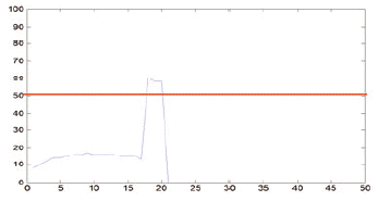
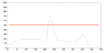
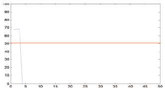
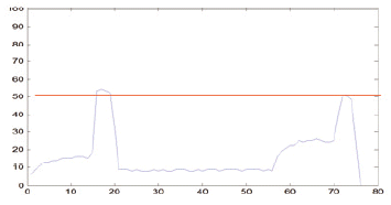
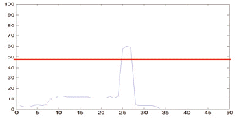
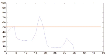
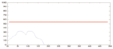
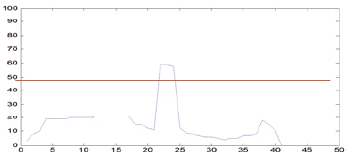
For each symbol image achieved after segmentation, we used vertical projection to obtain the histogram of this symbol, the base on the feature of line with the number of pixels. We also set some thresholds to find out the local peaks. By experimental, Threshold τ for vertical lines based on the height of staff line and the distance between lines are estimated by:
where, rH, rSr are the distance between lines and line height, respectively, and α, β are user-defined values.
According to the acknowledgement about music score rules, the length of vertical lines always smaller than the bar line (includes 4 * rH and 5 * rS) and bigger than half of the bar line. As such, in this work, we selected α, β as 2 and 3, respectively, to ensure that all of the vertical lines are precisely collected. Therefore, the interesting positions where a black note or white note could appear are where the vertical lines are located. As can be seen in Table 2, the red horizontal line, which was calculated from Eq. (1), is the threshold for detecting the vertical line of symbols after vertical projection. With a proper threshold the quarter note, bar line, sixteenth note, half note, and eight note get one vertical line. The multi note and beam note get two lines and sharp with the number of line equaling to zero.
3.3.2 Head note detection
Template matching for black note heads is applied for each vertical line position. The template is shifted in both sides of vertical line being equal to the distance between staff lines ( Fig. 3(a) and (b)). After this step, the number of lines and the number of head notes for each symbol are achieved. All symbols are categorized into 10 main classes for the next process.
3.4 SVM for Musical Symbol Recognition
After the first step, all of the symbols are divided into 10 main classes, some classes, such as the multi beam note, cleft include only have one subclass. We can ignore these main classes. Therefore, we only use seven SVMs for the rest of the seven main classes. Because SVM runs for each main class, the number of subclasses for each main class is small and we can limit the symbols that have similar shapes after segmentation. This will result in the performance being improved.
Eight SVMs are used for the same number of main classes. The two main classes of _BEAM_NOTE and SHARP_NATURAL apply binary classification to recognize two subclasses with a standard support vector machine algorithm. Since each main class contains more than two sub classes, the multiclass SVMs are implemented for recognition for the rest of the cases. With mobile devices, power is a serious issue. Therefore, to optimize our proposal method, we used the one–against–one method for classifying [ 17]. This means that for k subclasses that need to classify,
k(k-1)2 classifiers where each one is trained on data from two classes are constructed. Given l training data ( x1, y1), … , ( xl, yk), where xi ∈ Rn, i = 1, …, l, and yi ∈ {1,… k}, is the class of xi. For training data from the ith and jth subclasses, the binary classification problem shown below is solved as: Where, the training data xi are mapped to a higher dimensional space by the function θ. C is the penalty parameter,
ɛtij is the classification error, and wij, bij are parameters in the linear equation.
Minimizing12(wij)T is to maximize 2/||wij||, which is the margin between two groups of data.
C∑tɛtij is the term to reduce the number of training errors.
4. Experimental Results
To achieve the performance for musical symbol recognition, we used 22 music scores which captured from the camera with various morphologies: difference viewpoint, distortion, and illumination, as shown in Fig. 4. Then, two scenarios were used for implementation. After the segmentation step, all of the symbols were gathered and categorized into 10 main classes based on the number of head notes and the number of vertical lines. These symbol images were stored in 10 folders corresponding to the 10 main classes. Based on a specific scenario, the number of symbols for training and testing were then decided upon. Then, the SVMs were applied to the testing patterns to evaluate our proposed method’s performance. Multi SVMs were used to main multi-classes. Each class contains a small number of sub classes. Therefore, the time for training each main class is significantly reduced. The probability of confusion existing among the kinds of symbols is reduced appreciably.
The scenario one uses 22 music scores to collect all 2,273 symbols. The number of patterns for training takes two-thirds of the total symbols (1,538 symbols) and the rest of them spend to test (735 symbols). Table 3 shows the detail number for each class of symbols, as well as the total of testing and training number.
Table 4 shows the accuracy of Scenario 1. The first step of recognition is to classify all of the symbols into 10 main classes using heuristic characteristics. This method is simple and fast to implement. Then SVMs are applied for each main class with a small number of subclasses. As such, the accuracy for each main class is very high as well as the average accuracy of our method (99.2%) in Table 5.
We wanted to investigate the accuracy of our method in different scenes to evaluate the performance. So in Scenario 2, we used 22 music scores that were captured on camera. However, we used 12 scores for training and the rest were used for testing. The detail number of the patterns for each main class, the subclass, and the accuracy for each main class and average is showed in Tables 6 and 7. For Scenario 2, the training and testing symbols were collected independently from 22 music scores (12 scores for training and 10 scores for testing). So the symbols for testing can differ greatly to the training. Therefore, the accuracy is smaller than it was for Scenario 1. With more training, the accuracy would be higher.
To compare to the previous methods (using the learning machine methods to recognize all symbols directly), we ran SVM, NN with our database (according to [ 8], SVM and NN are the best methods for scanned and printed music score recognition). The accuracy in Fig. 5 shows that our proposal had the highest performance rate for music scores captured on camera.
5. Conclusion
In this paper, we introduced a new approach to recognize musical symbols extracted from music scores captured on camera with a different viewpoint, distortion, and illumination. The recognition process include heuristic acknowledges for splitting all symbols into subclasses before using SVM. The experimental results show that our method performs well. Based on the way to choose the set of training and testing, the accuracy could change. In our next work, we will continue to conduct research on this field, in order to improve the performance for all scenes.
Acknowledgement
This research was supported partly by Basic Science Research Program through the National Research Foundation of Korea (NRF) funded by MEST (2014-024950) and by the technological innovation R&D Program of SMBA (S2173771). Also this work was supported by SAMSUNG Electronics Co., LTD.
Biography
Tam Nguyen
She received B.S. degree in School of Electronics and Telecommunications from Hanoi University of Sciences and Technology, Vietnam in 2011. Since 2012, she has been taking the M.S. course in Electronics & Computer Engineering at Chonnam National University, Korea. Her research interests are mainly in the field of image processing, computer vision.
Biography
He received the B.S. degree in Electrical Engineering from Seoul National University in 1980. In 1982, he received the M.S. degree in Computer Engineering from Seoul National University. In 1991, he received Ph.D. degree in Computer Science from Pennsylvania State University. He is currently a professor of the Department of Electronics and Computer Engineering in Chonnam National University, Korea. Research interests image processing, computer vision, and video coding.
References
1. GS. Choudhury, M. Droetboom, T. DiLauro, I. Fujinaga, and B. Harrington, "Optical music recognition system within a large-scale digitization project," in Proceedings of 1st International Symposium on Music Information Retrieval (ISMIR 2000), Plymouth, MA, 2000.
2. M. Droettboom, I. Fujinaga, and K. MacMillan, "Optical music interpretation," in Structural, Syntactic, and Statistical Pattern Recognition, Heidelberg: Springer, 2002, pp. 378-387.  3. SE. George, in Visual Perception of Music Notation: On-Line and Off-Line Recognition, Hershey, PA: IRM Press, 2005.
4. W. Homcnda, and M. Luckner, "Automatic knowledge acquisition: recognizing music notation with methods of centroids and classifications trees," in Proceedings of International Joint Conference on Neural Networks (IJCNN’06), Vancouver, Canada, 2006, pp. 3382-3388.
5. LJ. Tardón, S. Sammartino, I. Barbancho, V. Gómez, and A. Oliver, "Optical music recognition for scores written in white mensural notation," Journal on Image and Video Processing, vol. 2009, article no. 6, 2009.  6. G. Taubman, "Musichand: a handwritten music recognition system,"thesis, Brown University; Providence, RI: 2005.
7. KT. Reed, and JR. Parker, "Automatic computer recognition of printed music," in Proceedings of International Conference on Pattern Recognition (ICPR’96), Vienna, Austria, 1996, pp. 803-807.  8. A. Rebelo, G. Capela, and JS. Cardoso, "Optical recognition of music symbols," International Journal on Document Analysis and Recognition, vol. 13, no. 1, pp. 19-31, 2010.  9. P. Bellini, I. Bruno, and P. Nesi, "Optical music recognition: architecture and algorithms," in Interactive Multimedia Music Technologies, Hershey, PA: Information Science Reference, 2008, pp. 80-110.  10. H. Miyao, and Y. Nakano, "Note symbol extraction for printed piano scores using neural networks," IEICE Transactions on Information and Systems, vol. 79, no. 5, pp. 548-554, 1996.
11. L. Pugin, "Optical music recognition of early typographic prints using hidden Markov models," in Proceedings of the 7th International Conference on Music Information Retrieval (ISMIR 2006), Victoria, Canada, 2006, pp. 53-56.
12. L. Pugin, JA. Burgoyne, and I. Fujinaga, "MAP adaptation to improve optical music recognition of early music documents using hidden Markov models," in Proceedings of the 8th International Conference on Music Information Retrieval (ISMIR 2007), Vienna, Austria, 2007, pp. 513-516.
13. N. Luangnapa, T. Silpavarangkura, C. Nukoolkit, and P. Mongkolnam, "Optical music recognition on android platform," in Advances in Information Technology, Heidelberg: Springe, 2012, pp. 106-115.  14. T. Soontornwutikul, N. Thananart, A. Wantanareeyachart, C. Nukoolkit, and C. Arpnikanondt, "Optical music recognition on Windows Phone 7," in Proceedings of the 9th International Conference on Computing and Information Technology (IC2IT2013), Bangkok, Thailand, 2013, pp. 239-248.  15. P. Bellini, I. Bruno, and P. Nesi, "Optical music sheet segmentation," in Proceedings of the 1st International Conference on Web Delivering of Music, Florence, Italy, 2001, pp. 183-190.  16. S. Sheridan, and SE. George, "Defacing music scores for improved recognition," in Proceedings of the 2nd Australian Undergraduate Students’ Computing Conference, Melbourne, Australia, 2004, pp. 142-148.
17. VQ. Nhat, and G. Lee, "Adaptive line fitting for staff detection in handwritten music score images," in Proceedings of the 8th International Conference on Ubiquitous Information Management and Communication (ICUIMC’14), Siem Reap, Cambodia, 2014. 
Fig. 1
Music score which is scanned from printed sheet (a), a part of music score which is captured from mobile camera (b) with illumination and distort effects. 
Fig. 2
The overall model of our proposed method. 
Fig. 3
The template of head note (a) and the positions of window for shifting (b). 
Fig. 4
Music scores capture from camera. 
Fig. 5
The comparison between three methods in accuracy. 
Table 5
The average accuracy of our method in Scenario 1
|
Training number |
Testing number |
Total |
The accuracy |
|
1,538 |
735 |
2,273 |
99.20% |
Table 7
The average accuracy of our method in Scenario 2
|
Training number |
Testing number |
Total |
The accuracy |
|
1,538 |
735 |
2,273 |
95.36% |
|
