Rotational Wireless Video Sensor Networks with Obstacle Avoidance Capability for Improving Disaster Area Coverage
Article information
Abstract
Wireless Video Sensor Networks (WVSNs) have become a leading solution in many important applications, such as disaster recovery. By using WVSNs in disaster scenarios, the main goal is achieving a successful immediate response including search, location, and rescue operations. The achievement of such an objective in the presence of obstacles and the risk of sensor damage being caused by disasters is a challenging task. In this paper, we propose a fault tolerance model of WVSN for efficient post-disaster management in order to assist rescue and preparedness operations. To get an overview of the monitored area, we used video sensors with a rotation capability that enables them to switch to the best direction for getting better multimedia coverage of the disaster area, while minimizing the effect of occlusions. By constructing different cover sets based on the field of view redundancy, we can provide a robust fault tolerance to the network. We demonstrate by simulating the benefits of our proposal in terms of reliability and high coverage.
1. Introduction
Surveillance applications oriented toward critical infrastructures and disaster relief are very important applications that many countries have identified as being critical in the near future. While disasters could result in a tremendous cost to our society, access to environment information in the affected area, such as, damage level and life signals, has been proven crucial for relief operations. Given the chaos that occurs in the affected areas, effective relief operations highly depend on timely access to environment information. Sensor networks can provide a good solution to these problems through actively monitoring and providing well-timed reporting emergency incidents to the base station. Previously, Wireless Sensor Networks (WSNs) [1–3] have been proposed to gather useful information in disasters, such as earthquakes, volcano eruptions, and mining accidents.
Wireless Video Sensor Networks (WVSNs) [4–6] are an emerging type of sensor network that contains many sensors equipped with miniaturized cameras. They represent a promising solution in many human life areas and can serve a variety of surveillance applications. For example, after the occurrence of a disaster, the area of the affected region poses many dangers to the rescue team. In the considered scenario of post-disaster management, a helicopter in the area of disaster can drop a large number of video sensors. Using a network composed of this variety of sensors can assist rescue operations by locating survivors and identifying risky areas. This type of application of sensor networks can not only increase the efficiency of rescue operations, but also ensure the safety of the rescue crew. These video sensors collaborate with each other to reach a common objective that is to ensure the coverage of the area by transmitting video data to a common destination (sink), then to decision-making centers using transport networks.
A WVSN management faces different challenges such as reliability, high coverage, fault tolerance, and energy consumption [7–10]. In this paper we are interested in the coverage problem with fault tolerance. Our main objective is to ensure a high multimedia coverage of a region of interest with occlusion-free viewpoints by using rotational video sensors. These rotational sensors are now possible and can be used broadly in practice due to the progress made in recent years in miniature robotics and to the economically accessible price proposed by some manufacturers, such as Arduino [11]. The coverage problem was largely studied in WSNs. The existing works take into account just scalar data and use omnidirectional sensors [12–15]. Different from WSNs, in WVSNs the sensing range of a video sensor node is represented by its field of view (FoV) (described in Subsection 3.2). Consequently, its coverage region is determined by its location and orientation.
In order to ensure a successful completion of the issued sensing tasks, sensor nodes must be appropriately deployed to reach an adequate coverage level. Therefore, in this work, we consider that a sensor can face three different directions. Different ways to extend the sensing ability of a WVSN exist. The first way is to put several video sensors of the same kind on one sensor node, each of which faces a different direction. The second way is to equip the sensor node with a mobile device that enables the node to move around [16]. The third way that we adopted is to equip the sensor node with a device that enables the sensor node to switch to different directions.
After a random deployment of video sensors, in case damages are caused by disasters, we can lose some video sensors that cover a critical region of the area. Therefore, to ensure better coverage with fault tolerance perspective, we have to use redundant nodes to cover the failed sensor’s FoV. In this paper we propose two different enhanced cover set construction approaches for the one provided by [17]. The aim of the first one is to find the maximum number of cover sets to ensure fault tolerance, which is presented in the simulation results. The second one is based on quality of coverage in order to show how we can ensure high precision of the covered object, even if we use the FoV of redundant video sensors. Regarding the activity of video sensors during the operational lifetime of the network, we exploited the scheduling of the video sensor nodes that was proposed in [17]. The main objective in this paper is to provide a coverage model using rotational sensors with fault tolerance, which is contrary to our previous work [18] where we used the same concept but for energy efficiency purposes. The idea behind using a rotation function rather than mobility is that, first, the rotation feature enables video sensors to maintain their geographical position while adjusting their FoV. Second, it facilitates communication between neighbor sensors. Consequently, we don’t have to add an additional driving mechanism, which allows us to decrease the cost of video sensors and energy consumption. Furthermore, we also considered the existence of obstacles positioned randomly in front of video sensors. Therefore, some modifications in the mathematical formulations of the paper [18] were made with the purpose of considering the area coverage by taking into consideration obstacle management. After video sensor nodes are randomly deployed, before the cover set construction phase, each video sensor calculates its second and third direction using its first direction that the sensor faces when it is deployed. Finally, the video sensor switches to the best and occlusion-free orientation in order to ensure high area coverage in the sensing field. The obtained results show that the proposed approach outperforms the already existing model [17] and another distributed coverage algorithm presented by [19] in terms of coverage by minimizing the effects of occlusion. This is mainly due to obstacles and takes into account fault tolerance in the network since more cover sets have been found.
The remainder of the paper is organized as follows: Section 2 elaborates the challenges of WVSN deployment for post-disaster management. Section 3 presents some related studies in the area of coverage with WVSN and the original video sensor node model. Section 4 describes the proposed rotational video sensor node model with obstacle avoidance capability. Section 5 addresses different cover set construction strategies and video sensor nodes’ scheduling. In Section 6, simulation results are presented on how to further increase network coverage when video sensor nodes have a rotation feature. Finally, the paper is concluded in Section 7.
2. Challenges of WVSN Deployment
In the case of a disaster, such as an earthquake, it is important to have an accurate and up-to-date overview of the situation in real time.
In the scenario presented in Fig. 1, we present a situation of post-disaster management where 25 video sensor nodes are randomly deployed. Fig. 1(a) shows the first deployment of video sensor nodes. Here, the video nodes’ FoVs are limited to the first random direction of the camera. We observed that the critical regions of the area are not completely covered by sensors since the people situated in regions 2 and 4 are not covered. Fig. 1(b) illustrates the WVSN topology after each video sensor has selected another FoV if it’s better than the first one, in order to maximize the area coverage. As can be seen in this figure, with the second deployment, regions 2 and 4 are completely covered after the second configuration of video sensors.

Wireless Video Sensor Networks deployment scenario for post-disaster management. (a) First deployment and (b) second deployment after field of view selection.
Furthermore, the proposed model has the ability to avoid occluded regions from occurring during the initial deployment. As shown in Fig. 1(a), the presence of an obstacle in front of region 3 results in the occlusion of video node v1’s FoV. This kind of situation has been considered in the proposed FoV selection algorithm (see Section 4) to find the best orientation of deployed video sensors while avoiding occluded regions, as shown in Fig. 1(b). In this figure region 3 is covered by video node v2’s FoV, which is not occluded by an obstacle.
We have also proposed a fault tolerance technique for WVSN to ensure coverage reliability. A node failure in this kind of network can be an incorrect state of hardware as a consequence of the failure of a component caused by an environmental disaster. The sensor node failure should not influence the working of the WVSN. The network needs to operate even when some of the sensor nodes fail. In randomly deployed sensor networks with sufficiently high node density, sensor nodes can be redundant (nodes that sense the same region) leading to overlaps among the monitored areas. Therefore, if a video sensor does not work anymore, then redundant neighbor nodes can be activated and thereby ensure the coverage of different parts of the failed node’s FoV (see Section 5).
3. Coverage in WVSNs
In this section we present some related works in the area of coverage and describe the already existing video sensor node model.
3.1 Related Work
Typically, three different kinds of coverage in WVSN have been considered, which are listed below.
Known-targets coverage: where video nodes try to monitor a set of targets (discrete points).
Barrier coverage: where the aim is to achieve a static arrangement of nodes that minimize the probability of undetected penetration through the barrier.
Area coverage: this aims to find a set of video nodes in order to ensure the coverage of the entire area.
Most previous research efforts are based on the known-targets coverage problem [20–23]. In [23] the authors constructed different sets of sensor nodes and not have to cover all the targets. In [20], the authors used directional sensors where the main objective is to find a minimal set of directions that can ensure the coverage of a maximum number of targets.
The goal of the barrier coverage is to deploy a chain of wireless sensors in the barrier, which usually is a long belt region, to prevent mobile objects from crossing the barrier undetected [24,25].
In the area coverage, sensor nodes must be deployed appropriately to reach an adequate coverage level for the successful completion of the issued sensing tasks [26–28]. The work presented in [29] use directional sensing models to achieve some given coverage probability requirements.
The majority of studies regarding multimedia sensor coverage consider an obstacle-free sensing environment. In [30], the authors described the area-coverage enhancement problem as maximum directional area coverage (MDAC). Kandoth and Chellappan [31] proposed a greedy solution called the face-away (FA) algorithm to achieve the maximal area coverage rate in the interested region. The authors in [32] enhanced the greedy algorithm proposed by [31] to improve the performance of the FA algorithm. Huang et al. [33] focused on the multimedia image sensor networks and proposed a virtual potential field-based method with the considerations of sensor direction and movement for the coverage enhancement. The authors in [19] proposed a distributed Voronoi-based self-redeployment algorithm (DVSA) to deal with the enhancement of the overall coverage ratio in the sensing field of a directional sensor network, which consists of mobile and rotational directional sensors. The authors used a Voronoi diagram to determine the sensing directions of sensors. In terms of the occlusion effect, Tezcan and Wang [34] presented an algorithm that enables self-configurable sensor orientation calculation. The goal is to find the camera orientation that minimizes occlusion viewpoints and overlapping areas.
In the proposed solution, we study the area coverage problem with the existence of obstacles by using a WVSN. Different from the above mentioned studies, in this work we propose a new distributed algorithm because it is computationally more scalable and does not incur high communication overhead, as required by a centralized algorithm. Furthermore, we focus on how to avoid obstacles by finding the most beneficial orientation for the video sensors that have the capability to rotate in three different directions. We are limited to three directions because in our application, we have to deploy a large number of low-cost multimedia sensors equipped with miniaturized cameras and which are limited in terms of computation, storage, and energy. Different from the work presented in [34], our objective is not to minimize the overlapping area. In contrast, we have taken advantage of overlapped FoVs in order to construct cover sets (see Section 5) and to use the scheduling algorithm proposed by [17] to ensure the maximum coverage of an area either by the video node itself or by a subset of its neighbors. This approach allows us to guarantee more reliability and fault tolerance in the proposed model.
3.2 Video Sensor Node Model
In WVSNs, the sensing range of sensor nodes is replaced with the camera’s FoV. The FoV, as illustrated in Fig. 2, is defined as the maximum volume that is visible from the camera. Therefore, the camera is able to capture images of distant areas and objects that appear within the camera’s FoV, which is the distance between the nearest and the farthest object that the camera can capture sharply.
Video sensor node model.
The FoV of a video sensor node v is defined as a sector denoted by a 5-tuple v(P,Rs, V⃗, α,d) where:
P refers to the position of video sensor node v (located at point P(p.x, p.y)),
Rs is its sensing range,
V⃗ refers to the vector representing the line of sight of the camera’s FoV, which determines the sensing direction,
α is the offset angle of the FoV on both sides of V⃗ (an angle of view [AoV] is represented by 2α),
d refers to the depth of view of the camera.
4. Rotational Video Sensor Node Model with Obstacle Avoidance
In order to enhance the coverage model presented above, we have added to each deployed sensor node in the area the capability to change its FoV. This new function is added at the first step just after deployment before starting the cover sets construction phase and the video sensor nodes’ scheduling procedure.
To address the proposed solution, we need to make the following assumptions:
All video sensors have the same sensing range (Rs), communication range (Rc), and offset angle α.
Video sensors within the Rc of a sensor are called the sensor’s neighboring nodes.
The sensing direction of each video sensor is rotational.
Each sensor knows its location information and determines the location of its neighboring sensors by using wireless communications.
The target region is on a two-dimensional plane with the presence of obstacles.
Fig. 3 shows a rotational video sensing model. The point P is the position of the video sensor that can switch to three possible directions of V⃗1, V⃗2, and V⃗3.
Rotational video sensing model.
V⃗1 is the direction that the sensor faces when it is deployed and the shadowed sector above V⃗1 is the sensing region of the video sensor when it works in V⃗1.
The different points of the first FoV1 are calculated as described below.
First, we have to randomly select a direction of the starting angle t1, where:
Since we have the coordinates (px, py) of the sensor node and we have already chosen a depth of view d, we can then calculate the coordinates of the three following different points (illustrated in Fig. 2) in order to obtain the desired FoV:
After the first deployment, since we have the starting angle of the first FoV1 defined in Eq. (1), the video sensor can calculate the second and the third direction with their respective FoV using the following equations, respectively:
And, by using the geometry formulas presented above, we can calculate the second FoV2 and the third FoV3 of the video sensor node.
After a neighborhood discovery, in the first step the video sensor calculates the number of neighbors that can cover its respective FoV for each direction.
In the second step, the video sensor search possible FoV, which is affected by an obstacle (example of how an obstacle would affect a FoV is given in Fig. 3; here the occluded direction is the third one).
Since the video sensor node model that we have enhanced and that takes into consideration just one direction of a video sensor provides us the type of video sensors that can detect obstacles. So, we have used a Boolean function (obstacleList.intersects(Segment(FoV.p, FoV.v))) (see Algorithm 1, line 17), which comes back with a response of “true” if at least one segment from the obstacle list intersects with the line of sight of a FoV (Segment(FoV.p, FoV.v)).
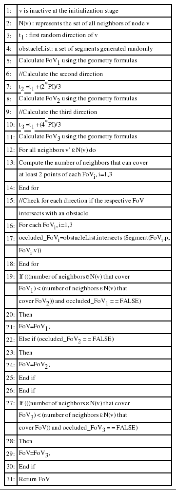
FoV selection
Finally, the video sensor switches to the direction that has the minimum number of neighbors without the existence of obstacles in order to ensure a maximum coverage and to avoid occluded regions. The procedure of the FoV selection is summarized in Algorithm 1.
We note that, Algorithm 1 generates n recursive calls in the worst case. Therefore, the time complexity of this algorithm is O(n), where n is the number of neighbor sensors of node v.

Simulation parameters
5. Cover Set Construction Strategies and Video Nodes’ Scheduling
For the purpose of surveillance applications, two different approaches can be used to enhance the cover set construction strategy. We explain each of them in the following sub-sections.
5.1 Coverage with Fault Tolerance
In the event of sensor failure, we can use redundant nodes that can cover the failed sensor node’s FoV by applying the cover set construction model to ensure fault tolerance. All of which is defined below.
Definition 1
A cover set Coi(v) of a video node v is defined as a subset of video nodes such that: ∪ v′ ɛ Coi(v) (v’s FoV area) covers v’s FoV area [17].
Definition 2
Co(v) is defined as the set of all the cover sets of node v [17].
In order to determine whether a sensor’s FoV is completely covered or not by a subset of neighbor sensors that are not occluded by obstacles, we proposed an enhancement of the approach defined by [17] where the aim is to use significant points of a video sensor’s FoV to determine cover sets. In the proposed cover set construction model, we have to select neighbor sensors that cover the points that are very close to the sensor’s barycenter (g) in order to get a higher number of cover sets and to avoid neighbors’ FoVs, but a high percentage of them have the possibility that two or more cover sets have some video nodes in common.
Note that we used the is_inside( ) feature of the extra graphical library defined by [17] to know whether a sensor’s FoV covers a given point. More details of this implementation are presented in Algorithm 2.
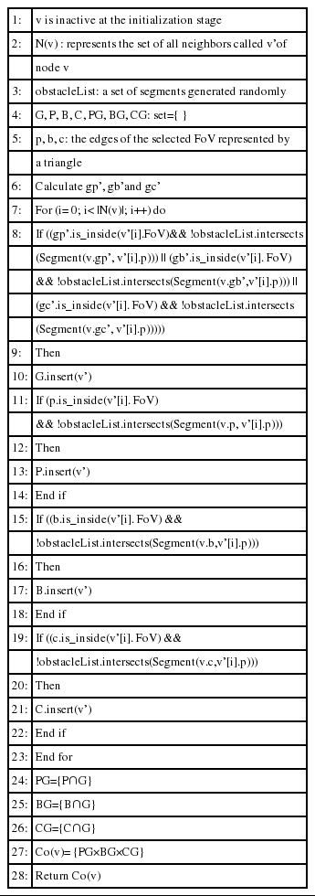
Cover set construction
In the example illustrated in Fig. 4, v’s FoV is represented by six points (p, b, c, gp’, gb’, and gc’). p, b, and c are the edges of the FoV represented by a triangle, gp’, gb’, and gc’ are the midpoints between the mid-point of their respective segments [pg], [bg], and [cg] and the barycenter g.
Example of cover set construction model.
To find the set of covers, node v has to find the following sets (at least one of the points (p, b and c) and another point gp’, gb’, or gc’):
PG = {v1, v4} where v1 and v4 cover the points p and gp’ of v’s FoV,
BG = {v3} where v3 covers the points b and gb’ of v’s FoV,
CG = {v2, v5} where v2 and v5 cover the points c and gc’ of v’s FoV.
Then, the node v can construct the set of cover sets (calculated by the Cartesian product of PG, BG and CG) as follows:
Co(v) = {{v},{v1, v3, v2}, {v4, v3, v2}, {v1, v3, v5}, {v4, v3, v5}}
In Algorithm 2, we note that the different sets of intersection generate n+m recursive calls in the worst case. Therefore, the intersection of two sets can be done with the complexity of O(n+m), where n and m are the cardinals of the two sets, respectively.
If we assume that the cover set {v1, v3, v2} is in active state and suddenly video node v1 fails due to a natural disaster, then another cover set, such as {v4, v3, v2}, can be selected to switch to an active state in order to ensure the coverage of the uncovered region.
5.2 Coverage with High-Accuracy
WVSNs are increasingly being used in different kinds of applications. However, traditional vision-based techniques for accurately calibrating cameras are not directly suitable for ad-hoc deployments of sensor networks in unreachable locations. Therefore, in scenarios where accurate camera calibration may not always be feasible and where we have to deploy video sensors with a very poor resolution camera, determining relative relationships between nearby sensor nodes may be the only available option.
In order to ensure area coverage with a high precision of the covered objects, we can enhance the cover set construction strategy by allowing a video sensor node to select only neighbors’ video sensor nodes that are very close to its barycenter.
In this approach we have to calculate the distance between the sensor’s barycenter (g) and the position p of each video sensor node included in the set of its neighbors after the neighborhood discovery.
First, we have to find the distance between the position p and the barycenter (g) of a video node v denoted by d(v.p, v.g), where:
Eq. (10) is added before line 7 (i.e., before the loop) in Algorithm 2 because it only concerns the coordinates of the sensor node.
We denote the distance between the position p of the neighbor v’ of video node v and the barycenter (g) of this last one by d(v’.p, v.g), where:
We have to add Eq. (11) after line 7 in Algorithm 2 in order to calculate this distance according to each neighbor node.
Finally, the selected neighbors’ video sensors to be included in the video node v’s cover set have to verify that:
Condition (12) is added after Eq. (11) to keep just the interesting neighbors video sensor nodes in the cover sets.
In this scheme, the selected video sensors for covering the video sensor that will be turned in the sleep mode are always the well-positioned sensors that have the best AoV, in order to improve the detection capabilities.
The only drawback of this cover set construction strategy is it can generate a lower number of cover sets compared to those generated by the already presented approach.
5.3 Rotational Video Sensor Nodes’ Scheduling
Regarding the rotational video sensor nodes’ scheduling, we have used the same algorithm proposed by [17]. Therefore, the activity of video sensor nodes operates in rounds as follows [17]:
Every node orders its set of cover sets according to their cardinality, and then gives the higher priority to the cover sets with the minimum cardinality.
If two sets or more in the cover sets have the same cardinality, then, priority is given to the cover set with the highest level of energy.
For each round, after receiving the activity message of its neighbors, the sensor node tests if the active nodes belong to a cover set. If so, it goes into the sleep state, otherwise (in the case that we have a node failure), it decides to be active and diffuses its decision.
6. Experimental Results
In this section, we present the simulation and analysis of the performance of the proposed scheme (denoted WVSN with rotational sensors [WVSNR]) by using the cover set construction strategy presented in Subsection 5.1. In order to address the coverage problem and to study the effect of the presence of obstacles in the area coverage, we have compared the proposed approach with the already existing model used in [17] (denoted WVSN), since it is based on the cover set construction approach. Some performance comparisons with another distributed algorithm [19] (denoted DVSA [mentioned in Subsection 3.1]) are also presented, so as to verify that the proposed approach can better enhance area coverage.
6.1 Simulation Environment
The effectiveness of the proposal is validated through simulations using the discrete event simulator OMNet++ [35]. Video sensor nodes have the same communication and sensing ranges. The position P and the direction V⃗ of a sensor node are chosen randomly. After a sensor node has received messages indicating the positions and directions of its neighbors, it can select an optimal direction that should not intersect with any obstacle in the field. The rest of the parameters are summarized in Table 1.
In order to study the impact of the network density on the performance of the proposed approach we varied the number of video nodes from 75 to 250.
In all simulation scenarios, random obstacles have been introduced to investigate occlusion issues and cause some area of the field to not be covered. A set of 25 obstacles represented by segments is positioned randomly at the initialization stage with a fixed sensing area.
Simulation ends when all active nodes of the network will have no neighbors.
To reduce the impact of randomness, we performed each simulation five times and then took the mean value.
6.2 Performance Metrics
We have used the three metrics explained below to compare the performance of the proposed approach.
Average percentage of coverage: refers to the average percentage of the area covered by the set of active nodes over the initial coverage area computed after the end of all simulation rounds.
Average number of cover sets: after the cover set construction phase, each node calculates the number of found cover sets. Then at the end of the simulation, statistics collected for the average number of cover sets for all the sensors are displayed.
Average percentage of active nodes: represents the average number of nodes involved in the active set over the initial number of the deployed sensors obtained by calculating the average percentage of active nodes. This percentage is obtained through different simulation rounds until the end of the network’s lifetime.
6.3 Performance Results
6.3.1 Average percentage of coverage
In the first step, we started simulations by computing the average percentage of coverage of the proposed WVSNR model compared with two existing approaches of WVSN and DVSA under the situations of varied network densities and sensing ranges. In the second step, we compared the proposed scheme only with the WVSN model by varying the communication range and considering the simulation duration time.
We can see from Fig. 5 that with a low network density (in the case of 75 and 100 sensor nodes), the DVSA model outperforms WVSN and WVSNR. The reason is that the DVSA uses the mobility function and that WVSNR, which is useful when we have a network, is not dense enough. However, when the number of sensor nodes exceeds 150, WVSNR performs better since only using rotation functionalities requires less of a response time and a quicker adjustment of sensors’ FoVs. We can also observe that the presence of obstacles severely affects the quality of coverage by using the model without rotation functionalities (WVSN). Since the proposed algorithm also decreases the obstacles’ detrimental effects by avoiding occluded FoVs, these enhancements allow us to obtain a significant improvement of coverage performance.

Average percentage of coverage by varying the network density. WVSN=Wireless Video Sensor Network, DVSA=distributed Voronoi-based self-redeployment algorithm, WVSNR=WVSN with rotational sensors.
We will now present the results obtained by varying the sensing range from 10 to 25 m with a fixed network density of 150 sensor nodes. When the sensing range increases, we can see in Fig. 6 that the average percentage of coverage also increases. We obtained a more interesting result using the WVSNR model compared with the existing WVSN and DVSA models. The reason is that in the proposed model we have to select only FoVs that are not obscured with obstacles and we always choose the direction at first to cover the less covered region by other sensors.

Average percentage of coverage by varying the sensing range. WVSN=Wireless Video Sensor Network, DVSA=distributed Voronoi-based self-redeployment algorithm, WVSNR=WVSN with rotational sensors.
In Fig. 7, the number of nodes is fixed one time at 150 and a second time at 250 video sensors for various communication ranges from 30 to 90 m. When the communication range increases, we can see that the average percentage of coverage also increases. This is because the larger the communication range is, the more sensing neighbors a sensor node will have. This will lead to obtaining a greater number of cover sets, especially for high density (the case of 250 sensors) where we have more communication between sensors.

Average percentage of coverage by varying the communication range. WVSNR=Wireless Video Sensor Network with rotational sensors.
Fig. 8 shows the average percentage of coverage for different simulation times with a network density of 100 sensors and a higher network density of about 200 sensors. Since simulation time ends when all active nodes have no neighbor, we can then evaluate the percentage of coverage with respect to the simulation time to have the longest network lifetime as a result. We can see from Fig. 8 that by using a network density of 200 sensors in the proposed approach the longest simulation time is obtained compared to the original model with a lower network density of 100 sensors.

Average percentage of coverage with respect to the simulation time. WVSNR=Wireless Video Sensor Network with rotational sensors.
6.3.2 Average number of cover sets
Fig. 9 shows the relationship between the average number of cover sets and the network density. The results presented in this figure indicate that the average number of cover sets increases almost linearly when the number of video sensors increases. The number of cover sets a sensor node can have depends on the network density and on the randomly set line of sight at each simulation run. It should be noted that the increase in the number of video sensors can lead to finding more cover sets in the case of the proposed scheme, which is useful for providing fault tolerance. We have found a lower number of cover sets using the model without rotation functionalities. The reason is that the presence of obstacles limits the FoV of respective nodes and with such obstructed FoVs the chances of FoVs overlapping with each other are reduced.
Average number of cover sets by varying the network density. WVSN=Wireless Video Sensor Network, WVSNR=WVSN with rotational sensors.
6.3.3 Average percentage of active nodes
From the results shown in Fig. 10, we can observe that increasing the network density (more than 100 sensor nodes) decreases the percentage of active nodes since we have more communication between the different nodes in the network.

Average percentage of active nodes by varying the network density. WVSN=Wireless Video Sensor Network, WVSNR=WVSN with rotational sensors.
We noticed that the network size has an impact on the node energy level and the effectiveness of the proposed model is shown in a large network since we obtained a greater number of cover sets with occlusion avoidance. These results are very interesting in the event of node failure since we have more other nodes that can ensure the coverage of the failed sensor nodes.
6.3.4 Impact of the offset angle α on the average percentage of coverage
We have also examined the effect of varying the AoV from 30° to 90° on the proposed model. Simulation results illustrated in Fig. 11 reveal that a large viewing angle of even 90° allows for obtaining better coverage than other AoVs. This is because using video sensors with a larger AoV increases the covered area. It can be observed in the proposed solution that using a greater network density and AoV allows us to avoid an uncovered sensing area and to ensure a maximal coverage.

Impact of the offset angle α on the average percentage of coverage. WVSN=Wireless Video Sensor Network, WVSNR=WVSN with rotational sensors.
6.3.5 Impact of the offset angle α on the average number of cover sets
Fig. 12 shows the relationship between the network density and the average percentage of cover sets by varying the AoV from 30° to 90°. From the simulation results illustrated in this figure, it can be observed that increasing the AoV leads to an increasing number of cover sets because with a larger FoV we can cover more points in the sensing area. Unfortunately, due to the cost of video sensors, low-resolution cameras embedded in wireless sensors will typically have a limited viewing angle in real-world implementations. Consequently, since it is more useful in the proposed model to use a WVSN with a large number of video sensors it is preferable to choose a limited AoV of the deployed sensors.
Impact of the offset angle α on the average number of cover sets. WVSN=Wireless Video Sensor Network, WVSNR=WVSN with rotational sensors.
7. Conclusions
In several surveillance applications and, more particularly, in post-disaster applications, the existence of obstacles is unavoidable. Therefore, the impact of obstacles is an inherent consideration to be brought in this kind of applications while designing a realistic coverage model. In this paper, we have proposed that a WVSN model be used in the situation of collecting post-disaster information. We studied the deployment of video sensor nodes by adding the capability of rotation for providing a better multimedia coverage, as well as other features, such as fault tolerance. A self-organized distributed algorithm has been proposed to enhance the coverage quality in a given area with obstacles. Different cover set construction strategies have been provided to rearrange connected cover sets in the presence of an unpredictable node failure to satisfy coverage criteria and to improve the fault tolerance. Simulation results indicate that the proposed approach performs better in area coverage with a higher percentage of coverage, even in the presence of obstacles in the considered region of interest.
As for future work, we will extend the experiments by including the comparison of additional approaches with more details concerning performance evaluation. It is also useful to address the effect of the number, shape, and position of obstacles on post-disaster applications and to show gains from this future study. Finally, we plan to evaluate the proposed model using field experiments.
References
Biography
Nawel Bendimerad http://orcid.org/0000-0001-6540-3431
She is a teacher at the National Polytechnic School of Oran and a researcher at Oran University, Algeria. She is a Ph.D. candidate at final stage. She received a M.S. degree (Magister) in computer science from Oran University in 2010. Since 2008 she has been doing research in wireless ad hoc and sensor networks. She has published six papers in refereed conference proceedings. Her current research area focuses on routing, energy consumption, quality of service, and security considerations in wireless video sensor networks.

Bouabdellah Kechar http://orcid.org/0000-0001-8635-4667
He is an assistant professor in the Department of Computer Science at Oran University, Algeria where he received his Ph.D. in 2010. He has authored several journal publications, refereed conference publications and one book chapter. He has been a member of the technical program and organizing committees of several international IEEE/ACM conferences and workshops. His current research interests include mobile wireless sensor/actuator networks, Zigbee/IEEE 802.15.4 technologies deployment, vehicular sensor networks and heterogeneous wireless networks, with special emphasis on radio resource management techniques, performance modeling, provisioning QoS and practical societal and industrial applications.
