Viewpoint Unconstrained Face Recognition Based on Affine Local Descriptors and Probabilistic Similarity

Article information

Abstract

1. Introduction

Face recognition has been widely investigated for the last decades, especially for robust face recognition algorithms that are able to deal with real world face recognition, such as identifying individuals from surveillance cameras for public security and annotating people from digital photos automatically. There are some successful commercial face recognition systems available like Google Picasa and Apple iPhoto [1]. However, face recognition research is still far from mature. Earlier face recognition algorithms are only effective under controlled settings, such as the probe and gallery images are frontal. This algorithm fails when it is applied to cases as pose and illumination changes. This paper focuses on the viewpoint invariant face recognition, which identifies a face when probe faces are from different viewpoints, while gallery faces are frontal.

The key issue for face recognition under different viewpoints is the distance between different poses is bigger than the distance between different subjects. One solution is to eliminate the distance between different poses. From among which, face normalization is an effective method to remove the difference in poses. Face normalization can be used as 2D or 3D models. As for the 2D model, Markov random fields (MRFs) are widely used to find correspondences between the frontal face with the profile probe faces [2,3]. MRFs find 2D displacement by minimizing the energy, which consists of two parts, one is the distance of the corresponding node and the other one represents the smoothness between neighbor nodes. The Lucas-Kanade method is also used for face alignment [4,5]. As for the 3D model, Blanz and Vetter [6] propose an effective 3D morphable method to fit the 3D model to a 2D face, and the fitting shape and texture coefficients were used to recognize faces. The normalization method can be used to construct the frontal face from the probe profile face [2]. It can also be used to directly match between images and the matching score, which represents the similarity between them [3]. These normalization methods are reported as being effective at the cost of a long computation time. It has been reported that two minutes was needed to normalize one face [2]. Marsico et al. [7] proposed a FACE framework to recognize a face for an uncontrolled pose and illumination changes. It detected some keypoints using the SIFT Active Shape Model (STASM) algorithm [8], and constructed a half face by the middle line key points. The rest of the face was reflected from the constructed half face. This easy method was fast, but not robust, because it highly depended on the accuracy of keypoint detection. When the keypoints detection failed, the system performances significantly decreased.

Another solution for face recognition under viewpoint change was to design a new classifier or a new feature. For the new classifier, one-shot similarity (OSS) or two-shot similarity (TSS) are proposed by introducing another dataset, which contains no probe and gallery images [9]. Each dataset contains different images of a single subject or different subjects viewed from a single pose. Similarity scores between two faces are calculated by the model built by one of the faces and the introduced dataset using Linear Discriminant Analysis (LDA) or Support Vector Machine (SVM). Cross-posed face recognition shares a similar concept by introducing a third dataset [10]. Faces from different viewpoints are all linearly represented by the introduced dataset using the subspace method. The similarity between these faces is then calculated indirectly by the linear coefficients. Recently, neural networks [11] and deep learning [12] have been adopted to extract pose invariant features for face recognition. As for new feature extraction, tied factor analysis is proposed to estimate the linear transformation and noise parameters in an ‘identity’ space [13]. The local descriptor is also an effective way to deal with affine transformation between two images, such as Harris-Affine [14], Hessian-Affine [15], and Affine SIFT [16] algorithms. Recently, the local Gabor binary pattern (LGBP) histogram sequence [17] and high-dimensional local binary pattern (LBP) [18] are proposed as effective local descriptors.

In this paper, we propose using the combination of Affine SIFT and Probabilistic Similarity for face recognition under a large change in viewpoint. In case of a large viewpoint variance, single local descriptors, such as SIFT and LBP, do not work well. The Affine SIFT algorithm tries to detect affine invariant local descriptors with the purpose of increasing the capacity of dealing with a significant pose change. However, the human face is not planar and it contains significant 3D depth. Affine SIFT doesn’t work effectively for large pose. To complement this, we combined it with probabilistic similarity, which gets the log likelihood between the probe and gallery face based on SSD distribution in an offline learning process.

The rest of this paper is organized as follows: Section 2 reviews the related work regarding the SIFT algorithm and image alignment. We describe the Affine SIFT algorithm and Probabilistic Similarity for face recognition and their combination ASIFT-PS in Section 3, respectively. Section 4 applies the ASIFT-PS to the FERET database, and presents the experiment results. Finally, we conclude this paper by explaining future work in Section 5.

2. Related Work

2.1 Scale Invariant Feature Transform

Local features are effective methods for conducting matching and recognition as it is robust against occlusion, scale, rotation, or even affine transformation to some extent. Among these algorithms, Scale Invariant Feature Transform (SIFT) is a scale and rotation invariant local feature. It transforms image data into scale-invariant coordinates and localizes the keypoint. Each keypoint is assigned to a descriptor. The major steps for the SIFT algorithm are as described below [19].

1. Scale-space extrema detection: An image is transformed into different scales and size. Extrema are searched by finding maxima and minima over all of scales using a difference of Gaussians scheme, which are invariant to scale and orientation.

   (1) D(x,y,σ)=(G(x,y,kσ)-G(x,y,σ))*I(x,y)

   where D(x, y,σ) is the difference of Gaussians function, G is the Gaussian function, σ is the scale of Gaussian, and k is the factor of nearby scales. I is the input image. Extrema are detected by comparing a pixel to its 26 neighbors at the current and adjacent two scales (8, 9, and 9 pixels for each scale, respectively) as shown in Fig. 1.

   

   Fig. 1

   Illustration of difference of Gaussian (DOG), octaves from bottom to top are generated by down-sampling. The initial image is convolved with Gaussian filter using different scales for each octave. Difference of Gaussian images is generated from this Gaussian filtered image. Extrema are localized by finding the maxima and minima comparing with neighboring pixels in the current scale and adjacent scales as shown on right.

2. Keypoint localization: Extrema are refined by excluding poor localized or low contrast points by checking the refined location, scale, and ratio of principal curvatures. This increases the stability of keypoint localization.

3. Orientation assignment: Each keypoint is assigned to one or more orientations based on a local image gradient histogram. To provide scale and rotation invariance, local image data is transformed to the corresponding orientation and scale for further keypoint descriptor calculations.

4. Keypoint descriptor: The local keypoint descriptor is calculated around each keypoint by the histogram of gradients. The descriptor is transformed into a representation that allows for significant levels of local shape distortion and change in illumination.

Fig. 1

Illustration of difference of Gaussian (DOG), octaves from bottom to top are generated by down-sampling. The initial image is convolved with Gaussian filter using different scales for each octave. Difference of Gaussian images is generated from this Gaussian filtered image. Extrema are localized by finding the maxima and minima comparing with neighboring pixels in the current scale and adjacent scales as shown on right.

A keypoint descriptor is created based on the gradient and orientation in a region around the center keypoint and a Gaussian window weights the region. The region is divided into 4×4 subregions, and the histogram of orientation with eight bins is accumulated for each subregion. Each orientation in the histogram corresponds to the sum of the gradient magnitudes near that direction.

There are several methods that have been proposed, such as best bin first (BBF) [20] and Hough transform [21], for image matching and recognition of the SIFT algorithm. The nearest neighbor is the original and effective matching method for SIFT features. SIFT features are first pre-extracted from gallery images and stored in a database. When matching with a probe image, each SIFT feature from the probe image is compared with all of the gallery features in a database. The nearest neighbor and second nearest neighbor are searched based on the Euclidean distance. The ratio of distances to the second nearest neighbor and nearest neighbor is compared with a threshold. The ratio that is smaller than the threshold is considered to be a matching face.

2.2 Image Alignment

Image alignment is used to find correspondences between two images. Among the algorithms of image alignment, the Lucas-Kanade algorithm is an effective one [4]. This algorithm starts from the non-overlapping division of an image into several subregions. Pixels in the same subregions have the same warp parameters. Let the warp function be X̄ = W(X, P) where X̄ is the coordinate of pixels of warped subregions with its corresponding pixel coordinate X = (x,y) of the original subregions. P = [p_1,p₂, …p_m]^T is the warp parameters with the dimension m. For the affine warp, m = 6, and:

(2) W(X,P)=(1+p1p3p5p21+p4p6) (xy1)

Let I and T represent the probe image and the gallery image, respectively. Fig. 2 shows these two images captured at two different poses. For each subregion r in T, we try to find a warp that aligns these two images. I_r is the corresponding subregion to T_r after warp transformation. The main objective of alignment is to minimize the error between the T_r and the warped subregions I_r as:

Fig. 2

Image to image alignment, an image is divided into several subregions T_r, a warp between two subregions T_r and I_r is calculated by minimizing the alignment error.

(3) Er=∑x(Ir(W(X,P))-Tr(X))2

The solution for Eq. (3) is to iterate calculating a ΔP and to update P until P converges. The Lucas-Kanade gives a solution for calculating ΔP by:

(4) ΔP=Himg-1∑x(∇Ir∂W∂P)T (Tr(X)-Ir(W(X,p)))

where ∇Ir=(∂Ir∂x,∂Ir∂y) is the gradient of I_r. ∂W∂P is the Jacobian of the warp (shown in Eq. (3)). H_img the pseudo Hessian matrix. We can now update the warp parameters P ← P + ΔP and iterate till the parameters P converge. This procedure is applied independently for every patch/subregion.

The warp between the probe image and gallery image can be learned online or offline. There are two kinds of online recognition methods. The first one is to calculate a match score for two images based on the warp parameters or alignment errors. Another one is to normalize images by transforming the profile face to its frontal face. Another scheme is off-line alignment. Warp parameters are trained from several sets of images and each set of images are from the same pose.

3. Proposed ASIFT-PS Algorithm

In this paper, we have proposed using the combination of the Affine SIFT and Probabilistic Similarity for face recognition. Affine SIFT is a stable and effective local descriptors for face recognition. However, the human face contains significant 3D depth. The performance of the Affine SIFT algorithm declines when a significant pose change exists. The Probabilistic Similarity (PS), which is the learning warp transformation between poses considering the 3D depth of a face, can provide complimentary information to the Affine SIFT in significant pose change. However, this alone is not distinctive enough since the warps vary from subject to subject. The combination of these two algorithms increases the capability of the system to recognize a face when there is a significant pose change.

3.1 Affine SIFT

The SIFT is the scale and rotation invariant feature, but it is not an affine invariant. The Affine SIFT is the extension of the SIFT algorithm. There are several parameters for affine transformation, which are:

(5) A=HλR1(ψ)TtR2(φ)=λ[cos ψ-sin ψsin ψcos ψ] [t001] [cos φ-sin φsin φcos φ]

where λ, R_i and T_t are a scale parameter, rotated angle, and tilted angle, respectively. Fig. 3 shows the geometric relationships of these parameters. The SIFT algorithm is just the scale (λ) and rotation (ψ) invariant. The other parameters t and φ are not invariant. Therefore, the SIFT algorithm is not fully an affine invariant. The Affine SIFT tries to fulfill the t and φ invariant, where t = 1/cosθ.

Fig. 3

Geometric relationship of affine decomposition. The λ and ψ are scale and rotation from camera. The θ and φ are tilt and rotation of subject, which named latitude and longitude, respectively.

The Affine SIFT transforms a frontal image into a series of simulated images by the change of longitude φ and latitude θ. These simulated images are sampled to achieve a balance between accuracy and sparsity. The ASIFT algorithm is as detailed below [16].

1. The latitude θ is changed to a geometric series 1, a,a² ,…, aⁿ, where a > 1. According to [16], a=2 is a good compromise between accuracy and sparsity. We also verified this by comparing the face recognition accuracy with various a from 1.5,2,2.5,3, and 2. The assignment of a=2 can achieve the best recognition accuracy. For a digital image, the tilt is conducted by a directional t-subsampling with an antialiasing filtered in advance, where t = 1/cosθ.

2. The longitude φ follows an arithmetic series for each tilt, as 0, b/t, …, kb/t, where b ≈ 72° achieves a balance, and k is the last integer satisfying kb/t < 180°.

3.3 ASIFT-PS Framework

In our framework, the Affine SIFT is first adopted to each gallery face (frontal face), and the probe faces use the SIFT algorithm. The Affine SIFT is used to detect keypoints and local features for the gallery face, and are stored in the keypoints database. For the recognition part, the SIFT algorithm is used to compute keypoints and local features for each probe face. This SIFT keypoints are compared with the Affine SIFT keypoints that are stored in the database. Let N be the total number of subjects to be recognized in the gallery. Each probe face is compared with these N subjects, resulting in a vector {M₁, ... , M_i, ... M_N} where M_i is the number of matching keypoints with subject i in the gallery.

In order to combine the PS algorithm, we need to first learn the υrw (log-means) and γrw (log-standard-deviations) of the SSD for cases that two faces belong to the same subject and not, respectively. In our experiment, we used half of the face images to train these parameters. Let N be the number of half training subjects. For each subregion r between a pair of poses, we have N pairs of the same subject and N*(N-1) pairs of different subjects. The SSD of these pairs are calculated separately from the same subject and different subjects. υrC and γrC are then obtained as the log-means and log-standard-deviations of the SSD of pairs with the same subjects. While υrI and γrI are the log-means and log-standard-deviations of the SSD of pairs with different subjects. Based on the υrC,γrC,υrI, and γrI we can calculate the probability similarity between a probe face with a gallery face using Eqs. (6) and (7). As a result, for N subjects to be recognized, a vector {L₁, ... , L_i, ... L_N}is obtained for each probe face, where L_i is the probability similarity with subject i in the gallery.

The final similarity between a probe face and a gallery face i is calculated as:

(8) Si=Mi+λ,(λ>0)

where M_i and L_i are the number of matching and probabilistic similarities with gallery image i. The λ is used to balance the value range between the matching number and probability. In our experiment, we varied λ from 1 to 15 with an interval of 1, and evaluated the face recognition rate. Fig. 4 shows the results with various λ and illustrates that λ = 10 can achieve a good performance.

Fig. 4

Face recognition accuracy with various λ from 1 to 15 with a step 1.

We can summarize our algorithm as follows:

Algorithm

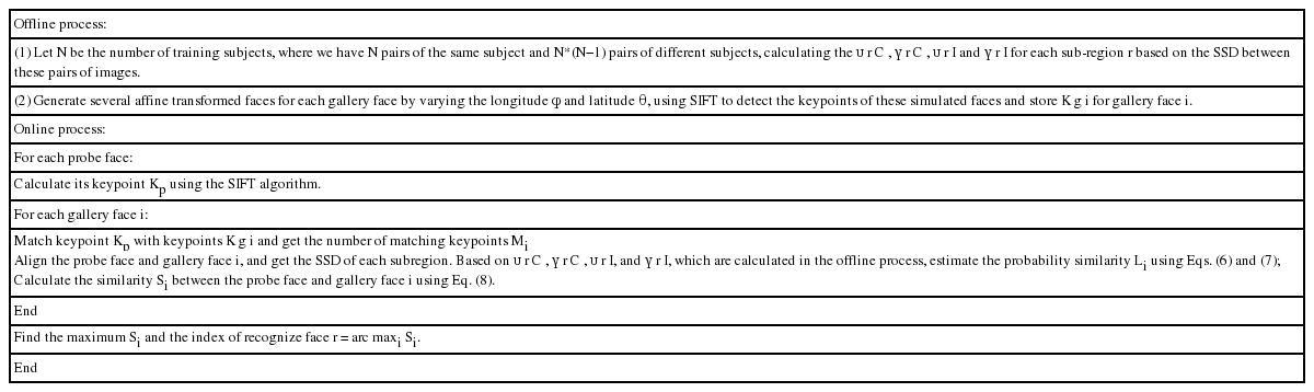
Face Recognition based on ASIFT-PS

4. Experimental Results

In our experiments, we used the FERET [22] grey database to evaluate our algorithm. This database contains 200 subjects and each subject contains nine images captured from different poses. For each subject, we used the frontal image as a gallery, and the other eight pose images as probe images, the pose angles of which are 60°, 40°, 25°, 15°, −15°, −25°, −40°, and −60°, respectively. These pose angles correspond to the horizontal viewpoint change from left to right. Fig. 5 shows these face images in the FERET database.

Fig. 5

Face images in FERET database with varying pose from (a) 0°, (b) 60°, (c) 40°, (d) 25°, (e) 15°, (f) −15°, (g) −25°, (h) −40°, and (i) −60°, respectively.

The proposed ASIFT-PS algorithm is compared with the LBP [23], LGBP [17], OSS [9], SIFT [19], Probabilistic Similarity [5], and ASIFT [16]. The parameters used in our experiment for the SIFT algorithm are as follows: the image is resized to a resolution of 400×400 and the ratio for the nearest neighbor is set to 0.8. For Probabilistic Similarity, the image is divided into 20×20 non-overlapping subregions for alignment. We used a CPU is Intel Core i7-4790 3.6 GHz, RAM is 8 GB to perform all of the experiments. The system that we used is a 64-bit Windows 7 Enterprise SP1.

We modified the original Affine SIFT so as not to spend computational time on invalid cases. We did this because the Affine SIFT generates a lot of viewpoints from a single frontal image. When setting the number of tilt to seven, the Affine SIFT generates 61 viewpoints. It takes too much time to match the keypoints with all of these viewpoints, and some of them are not that significant for face recognition because the face is detected only around special angles. Therefore, we restricted the viewpoints in a discrete series with only horizontal and vertical directions. This restriction would not reduce the performance much because the SIFT is effective when the pose difference is within 30 degrees. In our experiments, three and five viewpoints were examined in the horizontal and in the vertical direction. This results in a total of 15 viewpoints generated.

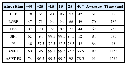
Table 1 shows the face recognition rate and computational time of face recognition with LBP, LGBP, OSS, ASIFT, SIFT, and PS on the FERET database. The computational time was calculated by averaging the matching time of each test face (Matching time is the time it takes to calculate one similarity). From among the compared algorithms, the ASIFT-PS achieved the best recognition performance and its computational time is the longest as well. However, it is worth noting that the computational time of ASIFT-PS does not have much of a difference with ASIFT, while the performance of ASIFT-PS is much better. We also noticed that SIFT could get similar results with ASIFT-PS when a pose degree was between −15° to 15°. However, ASIFT-PS achieved better results than SIFT or PS under a significant pose difference. The performance of the PS algorithm alone is not good. However, when combined with the ASIFT, the performance significantly increased. This is because the likelihood probability of the PS algorithm in a significant pose complement the performance deteriorates of ASIFT in large pose change. The ASIFT-PS algorithm didn’t increase the computational time by much because PS is performed in an offline manner. The face recognition rate was plotted for the FERET database in Fig. 6. The performance of PS was the worst. However, the ASIFT-PS, which is a combination of ASIFT and PS, showed the highest performance. It achieved about 10% in gains of recognition accuracy in the average under significant pose degrees.

Table 1

Comparison of recognition accuracy with SIFT, PS, ASIFT on FERET database

Fig. 6

Recognition rate of face with degrees varying from 60°, 40°, 25°, 15°, −15°, −25°, −40°, −60° in FERET database. Algorithms are Scale Invariant Feature Transform (SIFT), Probabilistic Similarity (PS), Affine-SIFT (ASIFT) and proposed ASIFT-PS.

5. Conclusions

In this paper, the ASIFT-PS was used for face recognition when a viewpoint change occurs. The Affine SIFT is an extension of the SIFT algorithm. The SIFT algorithm is the scale and rotation invariant, which is powerful for small viewpoint changes in face recognition. In our scheme, the Affine SIFT was only used for gallery faces, which generated a series of different viewpoints using affine transformation. In this way, it enabled viewpoint difference between gallery faces and probe faces. However, a human face is not planar and contains significant 3D depth. The Affine SIFT does not work well for a significant pose difference. The strength of the proposed method is that by combining the Affine SIFT and Probabilistic Similarity, the limitations of the Affine SIFT is eliminated and the Probabilistic Similarity’s statistical information compensates for the deficiencies of the SIFT algorithm. Thus, the accuracy of facial recognition increases by more than 10%, compared to other algorithms. To complement this, we combined the Affine SIFT with probabilistic similarity, which obtained the log likelihood between the probe and gallery face based on SSD distribution in an offline learning process. The FERET database was used to test the proposed ASIFT-PS. The results of our experiment showed that SIFT could achieve comparable results with the Affine SIFT when a pose degree was between −15° to 15°, but the ASIFT-PS achieved about 10% better on average as compared to SIFT under a large pose different.

Article information Continued