Xu and Xiao: Soft Set Theory Oriented Forecast Combination Method for Business Failure Prediction
Abstract
This paper presents a new combined forecasting method that is guided by the soft set theory (CFBSS) to predict business failures with different sample sizes. The proposed method combines both qualitative analysis and quantitative analysis to improve forecasting performance. We considered an expert system (ES), logistic regression (LR), and support vector machine (SVM) as forecasting components whose weights are determined by the receiver operating characteristic (ROC) curve. The proposed procedure was applied to real data sets from Chinese listed firms. For performance comparison, single ES, LR, and SVM methods, the combined forecasting method based on equal weights (CFBEWs), the combined forecasting method based on neural networks (CFBNNs), and the combined forecasting method based on rough sets and the D-S theory (CFBRSDS) were also included in the empirical experiment. CFBSS obtains the highest forecasting accuracy and the second-best forecasting stability. The empirical results demonstrate the superior forecasting performance of our method in terms of accuracy and stability.
Key words: Business Failure Prediction, Combined Forecasting Method, Qualitative Analysis, Quantitative Analysis, Receiver Operating Characteristic Curve, Soft Set Theory
1. Introduction
The current global business environment is increasingly complex, especially for venture capital providers. It motivates research to be carried out on business failure prediction (BFP) to deal with this situation [ 1]. Many statistical and intelligent methods have been proposed [ 2, 3]. For example, discriminant analysis [ 4, 5], logistic regression (LR) [ 6], probit regression [ 7], the case-based reasoning (CBR) method [ 8], neural networks [ 9], the genetic algorithm [ 10], rough sets [ 11], decision trees [ 12], the semi-parametric method [ 13], the discrete-time duration method [ 14], support vector machines (SVMs) [ 15], and the minimal optimization technique [ 16] were used for BFP. Since the pioneering work by Bates and Granger [ 17], many researchers have combined several forecasting methods together to improve forecasting performance [ 18– 23]. Most of the combined forecasting methods employed well-known combined methods including equal weighted, majority voting; Borda count; and Bayesian or intelligent algorithms, such as the neural network and fuzzy algorithm, as the combination method. However, as pointed out in [ 24– 26], there are many limitations in applying existing combination methods to combine individual forecasting methods for BFP. To overcome those limitations, Xiao et al. [ 25] employed the rough set and the Dempster-Shafer (DS) evidence theory as the combination method. Xiao et al. [ 24] used the fuzzy soft set as the weighted determination method. Li and Sun [ 22, 26] used an improved CBR as an individual forecasting method for BFP. Those methods may have good performance with samples of large sizes and certainty information. However, they are not good at dealing with small samples and soft and uncertain information [ 27, 28]. Besides, these combined methods also have a contradiction that the over-fitting problem may occur and the generalization power may be poor as the number of components increases. In this paper, to overcome those difficulties, we constructed a novel combined forecasting method for BFP. This method, named the combined forecasting method based on the soft set theory (CFBSS) combines with qualitative analysis and quantitative analysis for BFP to take full usage of the different types of information of each firm. CFBSS consists of three individual forecasting methods, which are the expert system (ES) method, LR, and SVM. This combination method is a novel technique, namely the soft set (SS) theory. Compared with other forecasting methods, the advantages of CFBSS are itemized as listed below.
CFBSS is good at dealing with not only large sample sizes, but also with small sample sizes. It is very useful for individual investors. The CFBSS has been developed based on the SS theory. Hence, it inherits the advantages of SS to deal with small sample sizes. CFBSS has an excellent adaptive capacity in the business environment. CFBSS combines with qualitative analysis and quantitative analysis for BFP. It has many advantages of dealing with qualitative, quantitative, and uncertainty information over statistical approaches, the fuzzy set theory, and so on. CFBSS does not have the contradiction where the over-fitting problem will occur and the generalization power will be poor as the number of components increases. Because SS is a parameterized family of subsets of the set U. For CFBSS, the weight coefficient is determined by a novel weight scheme, namely by the ROCB method, which is based on the receiver operating characteristic (ROC) curve [29]. It adaptively puts more weight on the component that produces a more accurate performance. CFBSS is easy to implement.
To compare the performance of CFBSS for BFP, we employed ES, LR, SVM, the combined forecasting method based on equal weights (CFBEWs), the combined forecasting method based on neural networks (CFBNNs), and the combined forecasting method based on rough sets and the D-S theory (CFBRSDS) as benchmarks. To test the influence of different sample sizes on the performance of forecasting methods, especially on the CFBSS, we divided all of the samples into training samples and testing samples with different percentages (20%, 80%) (50%, 50%) and (80%, 20%). Then, we did the empirical experiment separately. We carried out an empirical experiment using data sets collected from Chinese listed firms.
The remainder of the paper is organized as follows: Section 2 reviews BFP models and the SS theory. Section 3 introduces our proposed forecast combination method and provides a detailed description of its algorithm. Section 4 contains the empirical part and in Section 5 we discuss the results of our experiments. Finally, we provide our conclusions in Section 6.
2. Literature Review
2.1 Brief Review of the Soft Set Theory
The soft set theory, initiated by Molodtsov [ 27], is a newly emerging tool for dealing with uncertain decision problems. Unlike the theory of probability, the fuzzy set theory and the interval mathematics, which have their own limitations in terms of the inadequacy of parameterization, the SS theory is free from such difficulties and is considered to be a more proper tool for dealing with uncertainty. Since Maij et al. [ 30] provided a more detailed theoretical study by defining the operation rules of soft sets, the SS theory has been greatly developed. The definition of SS [ 27] can be briefly introduced as explained below. A pair (F, E) is called a soft set over U, if and only if, F is a mapping of E into the set of all subsets of the set U. In other words, the soft set is a parameterized family of subsets of the set U. Every set of F(ɛ),(ɛ ∈ E) from this family may be considered to be the set of ɛ – elements of (F, E), or as the set of ɛ – approximate elements of the soft set.
Up until now, researchers in the field of SS have mainly placed their attention on theoretical research. They usually integrate other intelligence algorithms or theories to develop SS [ 31– 34]. They seldom work on the application of SS to practical problems and not to BFP. The research in this paper contributes to SS by filling this gap. First, we provide SS a new practical background. This paper can be viewed as a test of the practicality of SS, which is one of the properties claimed in [ 27]. Second, we broadened the research field of SS. We applied SS to combine a multi-classifier for BFP to achieve a better performance.
2.2 Brief Review of Combined Forecasting Models for BFP
Previous works of BFP seldom combine qualitative analysis and quantitative analysis [ 35]. They mainly focus on a quantitative analysis based on the financial data [ 18– 21, 25]. However, as pointed out in [ 35], qualitative analysis has its own advantages over quantitative analysis. Therefore, it will be a great improvement to include qualitative analysis to construct an effective combined forecasting method based on a proper combination method. Previous researchers paid little attention to the combination of multiple methods for BFP. Most of them have focused on individual forecasting methods or ensembles of two forecasting methods [ 25, 36]. However, as pointed out by Bates and Granger [ 17], if one chooses an appropriate combining technology, a combination with more classifiers might produce a better result. This is because different classifiers can deal with different types of information. It is a key step to select an effective method to combine different classifiers for combined forecasting. Most of the prior literature chose well-known combined methods such as equal weighted, majority voting; Borda count; and Bayesian or intelligent algorithms, such as the neural network and fuzzy algorithm, as the combination method [ 25, 37]. Nevertheless, the existing combination methods listed above have their own limitations [ 25]. Thus, this research contributes to BFP. First, we propose a novel SS method as the combining method to improve the BFP technique with different sample sizes. The soft set thepry has advantages in terms of being flexible to deal with practical problems [ 27]. Second, we combined qualitative analysis and the quantitative analysis for BFP. Both qualitative analysis and quantitative analysis have their own advantages. We expect a good performance of our method to combine them together. The empirical results confirm our intuition.
3. The SS-Based Combined Forecasting Method for BFP
3.1 Combined Forecasting Model
In this section, we propose a novel forecast combination method based on the soft set theory (CFBSS) for BFP. The principle of CFBSS is illustrated in Fig. 1. Assume that there are N ( n=(1,2,…, N))sample firms and I ( i=(1,2,…, I)) forecasting methods, where YN is the vector that represents the state of each sample, YNI is the matrix that represents the forecasting result of the I method of N samples, and YNS is the vector that is the combined result of YNI based on SS. YN, YNI, and YNS are showed in Formula ( 1): where,
where, λi is the weight coefficient of individual ith forecasting methods, and:
yn = 0 means the nth sample firm is in a state of failure in practice and yn = 1 means that the nth sample firm is in normal state in practice. yni = 0 means the ith individual forecasting method believes that the nth sample firm will be in a state of failure and yni = 1 means that the ith individual forecasting method believes that the nth sample firm will be in a normal state. yns = 0 means that the CFBSS result shows that the nth sample firm will be in a state of failure and yns = 1 means that the CFBSS result shows that the nth sample firm will be in a normal state.
There are three key points in the process of conducting CFBSS for BFP. One is the selection of individual forecasting methods. Another is the selection of the combination method, and the last one is the choice of weight coefficient λi. As mentioned above, the combination method is based on the soft set for its advantages. Thus, we will focus on the study of the other two key points.
3.2 Individual Forecasting Method Selection
The individual forecasting method plays an important role in the performance of the combined forecasting method. For BFP, each individual forecasting method, such as NN, CBR, ES, MDA, LR, SVM, and so on, has its advantages and disadvantages. On the one hand, we want to integrate more methods into the forecast combination procedure to use their advantages. There is, however, a contradiction in doing so. The complexity of the combined forecasting method will increase as the number of components increases. As a result, an over-fitting problem will occur and the generalization power will be poor.
However, SS does not suffer such a problem. This is because SS is a parameterized family of subsets of the set U. The increase of the number of E ( E is the set of individual forecasting methods) will cause SS to perform better [ 27]. To reduce the complexity of CFBSS, the three components seem to be well balanced between obtaining better forecasting performance and reducing model complexity. Furthermore, we wanted to conduct qualitative analysis and quantitative analysis for BFP. Thus, we selected at least one qualitative analysis method and one quantitative analysis method. We employed ES, LR, and SVM as individual forecasting methods for their advantages. ES is a nice qualitative analysis tool, LR is a good statistical approach, and SVM is an efficient and intelligent algorithm. All of them have been demonstrated to be successful tools for BFP [ 6, 35, 38].
3.3 Weight Determination Based on the ROC Curve
In this paper, to overcome the limitations of existing methods for determining weights [ 24], we constructed a new weighted method (ROCB) based on the ROC curve analysis theory. The ROC curve has been proved its efficacy in evaluating forecasting models [ 29]. The idea is that we put more weight on the component that produces more accurate results for the training sample data. The principle of the ROCB method is showed in Fig. 2. BFP is a typical binary classification problem, in which the outcomes are labeled as either positive (P) or negative (N). There are four possible outcomes from a binary classifier. If the outcome from a prediction is positive and the actual state is also positive, then it is called a true positive (TP). However, if the actual value is negative, then it is said to have a false positive (FP). Conversely, a true negative (TN) occurs when both the prediction outcome and the actual value are negative, and a false negative (FN) occurs when the prediction outcome is negative, while the actual value is positive. We defined the ratio ACC to measure the forecasting accuracy of a forecasting method, as shown in Formula ( 4): Suppose that W is the matrix whose entry wij (i=1,2,…,I; j=1,2,…, J≤N) represents the ACC of the ith forecasting method on the jth group of the testing sample, where J is the number of groups of training samples.
Then, we can obtain a vector W′=[w1, w2, …, wI], in which wi(i=1,2,…,I) is the mean of jth column elements. It is a more accurate measurement to show the forecasting ability of each individual forecasting method. That is:
Then we obtain the weight coefficient λi of each individual forecasting method as follows:
Our weight scheme adaptively puts more weight on a forecasting method with more rate performance according to the data it applies.
3.4 Algorithm
Based on the analysis mentioned above, the algorithm of CFBSS, which is proposed in this paper, is showed in Fig. 3 and is demonstrated as shown below. Details of the algorithm of the CFBSS are described as detailed below.
Step 1. Preprocess financial data
The actual financial data is divided into two groups by 10 times’ split on the data. One group of the financial data is named the training data set. The other is called the holdout data set for validation. We employed the proposed procedure to the training data sets. First, we needed to normalize the data to eliminate the difference of each variable. The function of normalization is defined as show in Formula ( 8): Where xnm is the original value of the mth variable for the nth firm and maxm, minm are the maximal value and minimal value of the mth variable for all firms, respectively.
Step 2. Obtain the forecasting results of ES, LR, and SVM
With the individual forecasting methods for ES, LR, and SVM, we obtained the matrix yNI, as showed in Formula ( 1). For ES, we treated a finance analysis organization as an expert. These types of organizations publish their research reports about listed firms. For a listed firm’s stock, they will give a recommendation based on their analysis. Their recommendation may be ‘buy,’ ‘sell,’ or ‘keep.’ In other words, feature xES represents ‘advice of the financial analysis organization’ for ES forecasting in this paper.
We considered the advice from several experts, rather than one expert, to reduce the prediction bias. Suppose that there are T ( t = (1,2,…, T)) experts, and T is an odd number. For samples, we got the matrix YNT to reflect the forecasting results of T ESs, as shown in Formula ( 9): We coded ‘buy’ as 1, ‘sell’ as -1, and ‘keep’ as 0.
ynES is the final forecasting result of the nth firm from ES, as shown in Formula ( 10): That is, if most organizations recommend buying or keeping a certain listed firm stock, ES predicts the firm as Not Specially Treated (NST). The connection between ‘buy or keep’ and ‘sell’ never happens because of the odd number of T.
For LR, please refer the work by Ohlson [ 6]. We forecasted a firm as NST if the estimated probability of y = 1 was greater than 0.5. For SVM, we used the radial basis function as the kernel function. For details about SVM, please see the paper by Min and Lee [ 38]. The optimal choice of parameter of the kernel function is determined by the cross validation on a grid search.
Step 3. Compute the ACC of each individual forecasting method
According to Formula ( 4), we can get the ACC of each individual forecasting method. With Formulas ( 5) and ( 6), the ACC mean of each individual forecasting method can be computed.
Step 4. Compute the weighted coefficient λi
According to Formula ( 7), we can get the weighted coefficient λi of each forecasting method.
Step 5. Combine forecasting results with the soft set theory.
Suppose that U is the set of firms ( U = { h1, h2, …, hn}) of interest and E is the set of forecasting methods ( E = { e1, e2, ···, ei}). Let F be a mapping of E into the set of all subsets of the set U. According to the definition of the soft set theory [ 27], a SS ( F, E) can be constructed. Then, we are able to obtain the tabular representation of ( F, E), as shown as Table 1. With the weight coefficient λi, we can get the weighted tabular representation of ( F, E), as shown in Table 2. According to the literature [ 25], we set the critical value as 0.5 to predict whether or not one firm will be a failure in the future. In other words, the mapping F of the soft set ( F, E) can be presented as Formula ( 11). where,
yn′ is the final forecasting value of the CFBSS for the nth firm. It means that if ysn ≥ 0.5, then
yn′=1, we forecast that the nth firm will be a success. If ysn < 0.5, then
yn′=0, we predict that the nth firm will fail in the future.
4. Empirical Research
4.1 Samples and Data
According to the benchmark of the China Securities Supervision and Management Committee (CSSMC), listed firms are categorized into two classes of Specially Treated (ST) and Not Specially Treated (NST). The benchmark is either the net profits in the recent two consecutive years or purposely published financial statements with serious false and misstatements. More specifically, we consider ST companies as firms that have had negative net profits in the recent two years.
We used real data sets from Chinese listed firms. The financial data was collected from the Shenzhen Stock Exchange and the Shanghai Stock Exchange in China. We randomly selected 100 NST samples and 100 ST samples from the Shenzhen Stock Exchange and the Shanghai Stock Exchange that ranged from the years 2000 to 2012 in China. Thus, for the percentages (20%, 80%), it means that there are 40 samples for training and 160 samples for testing. The percentages (50%, 50%) and (80%, 20%) have the same means. Therefore, the training sample size is different. We can clearly observe the influence of different sample sizes on the performance of methods.
For ES, the data from finance analysis organizations in China range from the years 2000 to 2012. At present, there are more than 100 organizations working on the forecast analysis of Chinese listed firms. We consulted five(T =5)finance analysis organizations as our Expert System. Those five companies were randomly selected from the organizations that have similar backgrounds and forecasting abilities. The five companies selected are as follows: CITIC Securities, SHENYIN & WANGUO Securities, HAITONG Securities, CMS, and INDUSTRIAL Securities. Their research reports can be downloaded from either their websites or from the website of Invest Today.
4.2 Features Selection
In this paper, the CFBSS consists of quantitative analysis and qualitative analysis. Consequently, the CFBSS possesses characteristics of quantitative analysis and qualitative analysis. As pointed out in Section 3, xES is the only feature for qualitative analysis. Thus, in the following, we will focus on the feature selection for quantitative analysis.
For quantitative analysis methods, the initial features include profit ability, debt ability, activity ability, growth ability, cash ability, and shareholder profit ability. There are a total of 36 variables listed in Table 3. Obviously, these variables are highly correlated. It was necessary to do feature selection to avoid multicollinearity. Stepwise LR was employed to do the model complexity reduction. Five variables are statistically significant for predicting business failure and the selected features are listed in Table 4.
4.3 Experiment Design
In this paper, the aim of an empirical experiment is to investigate whether CFBSS can obtain a better performance for BFP. All samples were randomly divided into two groups with the percentages (20%, 80%), (50%, 50%), and (80%, 20%). One is a training sample set and the other is the testing sample set. As pointed out by the research conducted in [ 39], forecasting the year t using the data from the year ( t – 2) or ( t – 3) is more difficult than using the data from the year ( t – 1). In this paper, we tackled this challenge. To investigate whether CFBSS can obtain a better performance for BFP, three individual forecasting methods (ES, LR, SVM) and three combined forecasting methods (CFBEW, CFBNN, and CFBRSDS) were employed as benchmarks. The framework of this experiment is shown in Fig. 4 and is demonstrated as show below. The details of the empirical experiment is described as explained below:
Step 1. Collect data and classify NST and ST firms. We randomly split this data into three groups for this experiment. One is the holdout data set that will be rejected. The other is the training data set and the last one is the testing data set. Step 2. With the training data set and the selected features, we separately obtained forecasting results using ES, LR, and SVM. Then, the forecasting results were CFBEWs, CFBNNs, CFBRSDS, and CFBSS. Step 3. The testing data set was used for evaluating each forecasting model and we obtained the ACC. Step 4. We then compared the prediction performance and finished.
5. Results and Discussion
5.1 Results
In this paper, we extracted 100 non-ST Chinese listed firms and 100 ST Chinese listed firms from the Shenzhen Stock Exchange and the Shanghai Stock Exchange from the years 2000 to 2012. We used the 10-fold cross validation approach to train and evaluate the models. The MATLAB software package (2012) and Statistical Product and Service Solutions (IBM SPSS ver. 20) were employed to obtain the selected financial ratios and were used to compare the performance of different forecasting models based on different financial ratios with the same samples.
We chose RBF as the kernel function for SVMs for its advantages [ 38]. Grid-search and cross-validation were used to search for optimal parameters’ RBF values based on training datasets. A back propagation neural network (BPNN) [ 25] was employed as the NN algorithm. We ran 20 experiments on the training data for NN prediction and selected the optimal set of experiment results as the outputs for NN prediction. Validation data was used to compare the forecasting accuracy of different models. The forecasting results obtained by ES, LR, SVM, CFBEW, CFBNN, CFBRSDS, and CFBSS with data for the year ( t – 2) and ( t – 3) for the percentages (20%, 80%), (50%, 50%) and (80%, 20%) are showed in Tables 6– 11. The accuracy of each forecasting method for BFP was computed with Formula ( 4). In this paper, we input the four following statistical indices of: mean value, median value, variance value and coefficient of variance. The statistical results were extracted from Tables 6– 11. The mean value and the median value were critical in assessing forecasting accuracy [ 40]. These two indices are shown in Figs. 5 and 6. Variance value and the coefficient of variance are critical for assessing forecasting stability [ 25]. Both are illustrated in Figs. 7 and 8.
5.2.1 Forecasting accuracy discussion
Analysis of forecasting accuracy for the year (t – 2)
From Tables 6– 8 and Fig. 5 with the data for the year ( t – 2), we can easily see that CFBSS has the highest mean and median for forecasting accuracy percentage than those of other forecasting methods. With the percentages changing from (20%, 80%) to (80%, 20%), the accuracy does not change a lot. It is around 85%, which is because SS has an excellent ability for BFP with different sample sizes. Moreover, ES outperforms the rest of the methods. The accuracy of ES is around 82%. This is understandable since ESs are professional practitioners and may have some more information. Agreeing with Li and Sun’s empirical result [ 21], the performance of the rest of the forecasting methods is quite different with different sample sizes. They all have an increasing higher accuracy with the percentages changing from (20%, 80%) to (80%, 20%). The size of the training sample is bigger and the accuracy is higher, especially for LR, CFBEW, and CFBNN. This is due to the fact that they have restrictions on sample sizes. For SVM and CFBRSDS, they have a higher accuracy than LR, CFBEW, and CFBNN when the sample size is small. This is because the SVM and D-S theory has weaker restrictions on sample sizes. Clearly, for the year ( t – 2), the sample sizes have a great effect on the forecasting accuracy of each method for BFP. However, CFBSS is an effective tool for BFP with different sample sizes. Without the limitation of sample sizes, combined forecasting methods have higher forecasting accuracy than individual forecasting methods. This is due to the fact that those methods utilize more information for BFP than individual forecasting methods, and that they been developed based on individual forecasting methods.
Analysis of forecasting accuracy for the year (t – 3)
From Tables 9– 11 and Fig. 6 with the data for the year ( t – 3), we can easily see that the conclusion is similar to the result for the data for the year ( t – 2). Thus, we focused on analyzing the difference between them. For each forecasting method for BFP, forecasting with data sets for the year ( t – 2) will have higher accuracy than forecasting with data sets for the year ( t – 3). This is the same result that was pointed out in [ 39]. This is due to the fact that with a longer amount of time passing before forecasting, there may be more unpredicted incidents happening. Furthermore, unpredicted incidents may affect firms’ operations. Thus, using this current information is not very efficient for BFP long after.
5.2.2 Forecasting stability discussion
Analysis of forecasting stability for the year (t – 2)
From Tables 6– 8, and Fig. 7 with the data for the year ( t – 2), we can easily see that ES has the smallest value in terms of the forecasting variance and coefficient of variance out of all of the employed forecasting methods mentioned above. This means that ES has the best forecasting stability than the other forecasting methods. This is because ESs are professional practitioners who pay more attention to forecasting stability. The second-lowest forecast variation method is CFBSS. With the percentages changing from (20%, 80%) to (80%, 20%), the value of the variance and coefficient of variance only differ within 1%. This is due to the fact that SS has an excellent ability for combining with qualitative analysis and quantitative analysis under different sample sizes [ 27]. The rest of the forecasting methods perform differently on the forecasting stability with the percentages changing from (20%, 80%) to (80%, 20%). Generally, the stability will be better with bigger sample sizes. However, when the percentage is (80%, 20%), the values of the variance and coefficient of variance of the forecasting methods are bigger than those with the percentages of (20%, 80%) or (50%, 50%). This goes against the commonly held view. However, this is understandable because when the percentages are (80%, 20%), in this paper, for 10-fold cross-validation, each testing group only has four samples. If there is a small change, the variance and coefficient of variance will change significantly. If there are enough samples, the situation is better. In the future, more work will be done on this.
Analysis of forecasting stability at year (t – 3)
From Tables 9– 11, and Fig. 8 with the data for the year ( t – 3), we can easily see that the conclusion is similar to the conclusion for the data for the year ( t – 2). Thus, we focused on analyzing their difference. For each forecasting method for BFP, forecasting with data sets for the year ( t – 2) will have a better forecasting stability than forecasting with data sets for year ( t – 3). This is in keeping with the result that was pointed out [ 25]. This is due to the fact that with a longer amount of time passing before forecasting, there may be more unpredicted incidents occurring. These unpredicted incidents will affect the operation of a firm. In other words, these unpredicted incidents are considered to be noise. Thus, using this current information is not very efficient for BFP long after.
5.2.3 Summary
Based on the analysis above, we can see that CFBSS, which has been proposed in this paper, has the highest forecasting accuracy and the second best forecasting stability over other forecasting methods with different sample sizes. In other words, this novel combined forecasting method of CFBSS, which combines qualitative analysis and quantitative analysis that is based on the SS theory, can improve the forecasting performance of BFP.
6. Conclusion
In this paper, we extended the research of forecast combination methods for BFP with different sample sizes by proposing a combined forecasting method of ES, LR, and SVM based on the SS theory. We introduced a new weighted scheme based on the ROC curve theory to obtain suitable weight coefficients of CFBSS. Compared with ES, LR, SVM, CFBEW, CFBNN, and CFBRSDS, our method demonstrates superior performance and a high stability for the BFP of Chinese listed firms.
Though the results are satisfactory, our proposed method has some limitations. The mapping function F that is employed in SS needs to be further developed. That is because these mapping functions will provide deeper insights to the forecasting performance of BFP. In our current work, we used ES, LR, and SVM as the components and set the number of ESs to 5. Doing so seems to be effective, but is based on heuristics. Systematical and theoretical developments on the selection of models are continuations of this work. Furthermore, the CFBSS obtained a good forecasting performance for the BFP of Chinese listed firms. We do not know its forecasting performance on financial data sets from other countries. It definitely deserves further exploration.
Biography
He received the B.A. degree in Logistic Management from Jiangxi University of Finance and Economic in 2008. Currently, he is a Ph.D. candidate in the School of Economics and Business Administration at Chongqing University. His research interests include intelligent decision-making, information intelligent analysis and business Intelligence.
Biography
Zhi Xiao
He received the B.S. degree in Department of Mathematics from Southwest Normal University in 1982. And he received his Ph.D. degree in Technology Economy and Management from Chongqing University in 2003. He is currently a Professor in the School of Economics and Business Administration at Chongqing University. His research interests are in the areas of information intelligent analysis, data mining, and business Intelligence.
References
1. G. Wang, J. Ma, and S. Yang, "An improved boosting based on feature selection for corporate bankruptcy prediction," Expert Systems with Applications, vol. 41, no. 5, pp. 2353-2361, 2014.  2. J. Sun, H. Li, QH. Huang, and KY. He, "Predicting financial distress and corporate failure: a review from the state-of-the-art definitions, modeling, sampling, and featuring approaches," Knowledge-Based Systems, vol. 57, pp. 41-56, 2014. 3. CC. Yeh, DJ. Chi, and MF. Hsu, "A hybrid approach of DEA, rough set and support vector machines for business failure prediction," Expert Systems with Applications, vol. 37, no. 2, pp. 1535-1541, 2010. 4. WH. Beaver, "Financial ratios and predictors of failure," Journal of Accounting Research, vol. 4, no. 4, pp. 71-111, 1966. 5. EI. Altman, "Financial ratios, discriminant analysis and the prediction of corporate bankruptcy," Journal of Finance, vol. 23, no. 4, pp. 589-609, 1968. 6. JA. Ohlson, "Financial ratios and the probabilistic prediction of bankruptcy," Journal of Accounting Research, vol. 18, no. 1, pp. 109-131, 1980. 7. HJ. Zmijewski, "Methodological issues related to the estimation of financial distress prediction models," Journal of Accounting Research, vol. 22, pp. 59-82, 1984. 8. SM. Bryant, "A case-based reasoning approach to bankruptcy prediction modeling," Intelligent Systems in Accounting, Finance and Management, vol. 6, no. 3, pp. 195-214, 1997. 9. M. Adya, and F. Collopy, "How effective are neural networks at forecasting and prediction? A review and evaluation," Journal of Forecasting, vol. 17, no. 5–6, pp. 481-495, 1998. 10. F. Varetto, "Genetic algorithm application in the analysis of insolvency risk," Journal of Banking and Finance, vol. 22, no. 10, pp. 1421-1439, 1998. 11. AI. Dimitras, R. Slowinski, R. Susmaga, and C. Zopounidis, "Business failure prediction using rough sets," European Journal of Operational Research, vol. 114, no. 2, pp. 263-280, 1999. 12. TE. McKee, and M. Greenstein, "Predicting bankruptcy using recursive partitioning and a realistically proportioned data set," Journal of Forecasting, vol. 19, no. 3, pp. 219-230, 2000. 13. RC. Hwang, KF. Cheng, and JC. Lee, "A semiparametric method for predicting bankruptcy," Journal of Forecasting, vol. 26, no. 5, pp. 317-342, 2007. 14. CW. Nam, TS. Kim, NJ. Park, and HK. Lee, "Bankruptcy prediction using a discrete-time duration model incorporating temporal and macroeconomic dependencies," Journal of Forecasting, vol. 27, no. 6, pp. 493-506, 2008. 15. W. Hardle, YJ. Lee, D. Schafer, and YR. Yeh, "Variable selection and oversampling in the use of smooth support vector machines for predicting the default risk of companies," Journal of Forecasting, vol. 28, no. 6, pp. 512-534, 2009. 16. YC. Hu, and J. Ansell, "Retail default prediction by using sequential minimal optimization technique," Journal of Forecasting, vol. 28, no. 8, pp. 651-666, 2009. 17. JM. Bates, and CW. Granger, "The combination of forecasts," Operations Research Quarterly, vol. 20, no. 4, pp. 451-468, 1969. 18. H. Jo, and I. Han, "Integration of case-based forecasting, neural network, and discriminant analysis for bankruptcy," Expert Systems with Applications, vol. 11, no. 4, pp. 415-422, 1996. 19. FY. Lin, and S. McClean, "A data mining approach to the prediction of corporate failure," Knowledge-Based Systems, vol. 14, no. 3, pp. 189-195, 2001. 20. J. Sun, and H. Li, "Listed companies’ financial distress prediction based on weighted majority voting combination of multiple classifiers," Expert Systems with Applications, vol. 35, no. 3, pp. 818-827, 2008. 21. H. Li, and J. Sun, "Majority voting combination of multiple case-based reasoning for financial distress prediction," Expert Systems with Applications, vol. 36, no. 3, pp. 4363-4373, 2009. 22. H. Li, JL. Yu, LA. Yu, and J. Sun, "The clustering-based case-based reasoning for imbalanced business failure prediction: a hybrid approach through integrating unsupervised process with supervised process," International Journal of Systems Science, vol. 45, no. 5, pp. 1225-1241, 2014. 23. CF. Tsai, "Combining cluster analysis with classifier ensembles to predict financial distress," Information Fusion, vol. 16, pp. 46-58, 2014. 24. Z. Xiao, K. Gong, and Y. Zou, "A combined forecasting approach based on fuzzy soft sets," Journal of Computational and Applied Mathematics, vol. 228, no. 1, pp. 326-333, 2009. 25. Z. Xiao, XL. Yang, Y. Pang, and X. Dang, "The prediction for listed companies financial distress by using multiple prediction methods with rough set and Dempster-Shafer evidence theory," Knowledge-Based Systems, vol. 26, pp. 196-206, 2012. 26. H. Li, and J. Sun, "Predicting business failure using an RSF-based case-based reasoning ensemble forecasting method," Journal of Forecasting, vol. 32, no. 2, pp. 180-192, 2013. 27. D. Molodtsov, "Soft set theory: first results," Computers & Mathematics with Applications, vol. 37, no. 4–5, pp. 19-31, 1999. 28. W. Xu, Z. Xiao, X. Dang, DL. Yang, and XL. Yang, "Financial ratio selection for business failure prediction using soft set theory," Knowledge-Based Systems, vol. 63, pp. 59-67, 2014. 29. T. Fawcett, "An introduction to ROC analysis," Pattern Recognition Letters, vol. 27, no. 8, pp. 861-874, 2006. 30. PK. Maji, R. Biswas, and AR. Roy, "Soft set theory," Computers & Mathematics with Applications, vol. 45, no. 4–5, pp. 555-562, 2003. 31. DG. Chen, ECC. Tsang, and DS. Yeung, "Some notes on the parameterization reduction of soft sets," in Proceedings of International Conference on Machine Learning and Cybernetics, New Orleans, LA, 2003, pp. 1442-1445.
32. Z. Xiao, L. Chen, B. Zhong, and S. Ye, "Recognition for soft information based on the theory of soft sets," in Proceedings of International Conference on Services Systems and Services Management (ICSSSM’05), Chongging, China, 2005, pp. 1104-1106.
33. DV. Kovkov, VM. Kolbanov, and DA. Molodtsov, "Soft sets theory-based optimization," Journal of Computer and Systems Sciences International, vol. 46, no. 6, pp. 872-880, 2007. 34. F. Feng, YM. Li, and N. Cagman, "Generalized uni-int decision making schemes based on choice value soft sets," European Journal of Operational Research, vol. 220, no. 1, pp. 162-170, 2012. 35. AI. Dimitras, SH. Zanakis, and C. Zopounidis, "A survey of business failure with an emphasis on prediction method and industrial application," European Journal of Operational Research, vol. 90, no. 3, pp. 487-513, 1996. 36. F. Lin, D. Liang, CC. Yeh, and JC. Huang, "Novel feature selection methods to financial distress prediction," Expert Systems with Applications, vol. 41, no. 5, pp. 2472-2483, 2014. 37. E. Kim, W. Kim, and Y. Lee, "Combination of multiple classifiers for customer’s purchase behavior prediction," Decision Support Systems, vol. 34, no. 2, pp. 167-175, 2002. 38. JH. Min, and YC. Lee, "Bankruptcy prediction using support vector machine with optimal choice of kernel function parameters," Expert Systems with Applications, vol. 28, no. 4, pp. 603-614, 2005. 39. H. Li, and J. Sun, "Forecasting business failure: the use of nearest-neighbour support vectors and correcting imbalanced samples: evidence from the Chinese hotel industry," Tourism Management, vol. 33, no. 3, pp. 622-634, 2012. 40. H. Li, and J. Sun, "Forecasting business failure in china using case-based reasoning with hybrid case respresentation," Journal of Forecasting, vol. 29, no. 5, pp. 486-501, 2010.
Fig. 1
The principle of the combined forecasting based on the soft set theory (CFBSS) method. 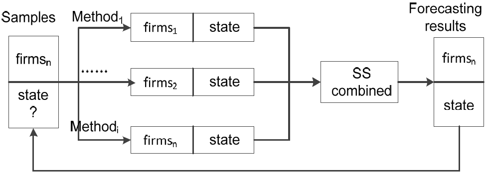
Fig. 2
Principle of the receiver operating characteristic curve based (ROCB) method. TP=true positive, TN=true negative, FP=false positive, FN=false negative, ACC=accuracy. 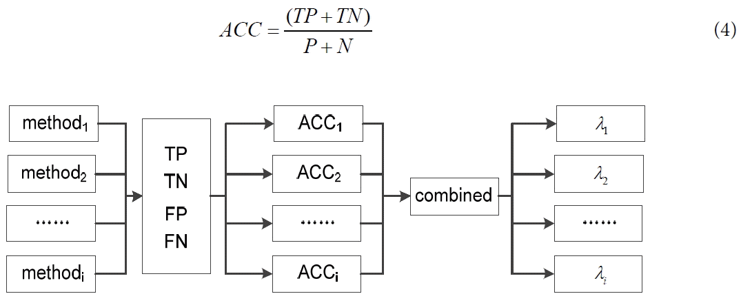
Fig. 3
The algorithm of the combined forecasting method based on the soft set theory (CFBSS).
ES=expert system, LR=logistic regression, SVM=support vector machine.
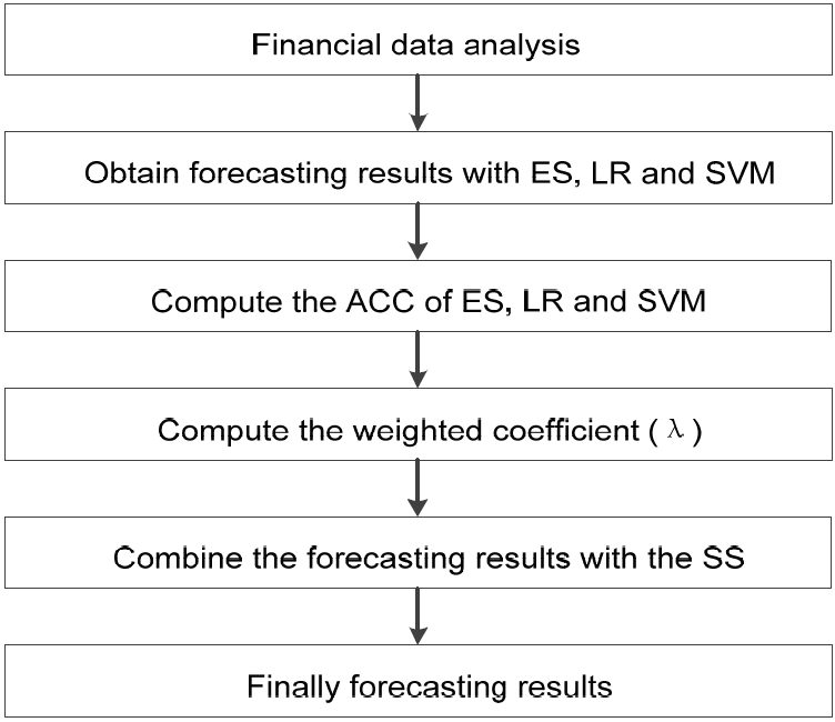
Fig. 4
Empirical experiment design. ES=expert system, LR=logistic regression, SVM=support vector machine, CFBEW=combined forecasting based on equal weight, CFBNN=combined forecasting based on neural network, CFBRSDS=combined forecasting based on the rough set and Dempster-Shafer evidence theory, CFBSS=combined forecasting based on the soft set theory. 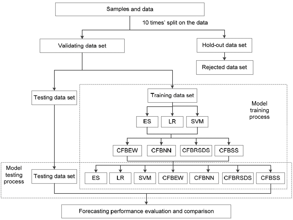
Fig. 5
Mean value and median value of forecasting results at year (t – 2). ES=expert system, LR=logistic regression, SVM=support vector machine, CFBEW=combined forecasting based on equal weight, CFBNN=combined forecasting based on neural network, CFBRSDS=combined forecasting based on the rough set and Dempster-Shafer evidence theory, CFBSS=combined forecasting based on the soft set theory. 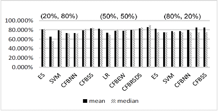
Fig. 6
Mean value and median value of forecasting results at year (t – 3). ES=expert system, LR=logistic regression, SVM=support vector machine, CFBEW=combined forecasting based on equal weight, CFBNN=combined forecasting based on neural network, CFBRSDS=combined forecasting based on the rough set and Dempster-Shafer evidence theory, CFBSS=combined forecasting based on the soft set theory. 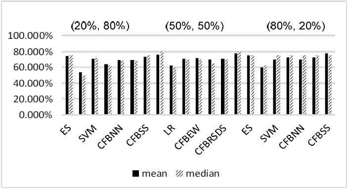
Fig. 7
Variance value and coefficient of variance value of forecasting results at year (t – 2). ES=expert system, LR=logistic regression, SVM=support vector machine, CFBEW=combined forecasting based on equal weight, CFBNN=combined forecasting based on neural network, CFBRSDS=combined forecasting based on the rough set and Dempster-Shafer evidence theory, CFBSS=combined forecasting based on the soft set theory. 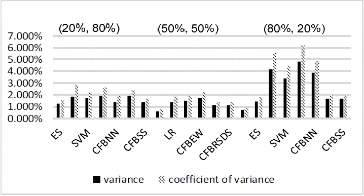
Fig. 8
Variance value and coefficient of variance value of forecasting results at year (t – 3). ES=expert system, LR=logistic regression, SVM=support vector machine, CFBEW=combined forecasting based on equal weight, CFBNN=combined forecasting based on neural network, CFBRSDS=combined forecasting based on the rough set and Dempster-Shafer evidence theory, CFBSS=combined forecasting based on the soft set theory. 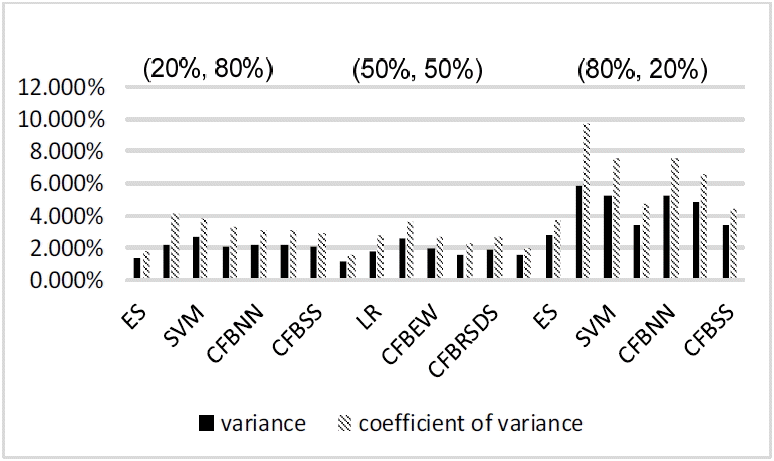
Table 1
Tabular representation of (F, E)
|
U
|
e1
|
··· |
eI
|
|
h1
|
y11
|
··· |
y1I
|
|
h2
|
y21
|
··· |
y2I
|
|
⋮ |
⋮ |
⋮ |
⋮ |
|
hN
|
yN1
|
··· |
yNI
|
Table 2
Weighted tabular representation of (F, E)
|
U
|
(e1,λ1) |
··· |
(eI, λI) |
ysn
|
|
h1
|
y11
|
··· |
y1I
|
ys1=∑i=1Iλiy1i
|
|
h2
|
y21
|
··· |
y2I
|
ys2=∑i=2Iλiy2i
|
|
⋮ |
⋮ |
⋮ |
⋮ |
⋮ |
|
hN
|
yN1
|
··· |
yNI
|
ysN=∑i=1IλiyNi
|
Table 3
|
No. |
Financial ratio |
No. |
Financial ratio |
|
X1
|
Net operating income rate |
X2
|
Net profit to current assets |
|
X3
|
Net profit to total assets |
X4
|
Net profit to fixed assets |
|
X5
|
Net profit to equity |
X6
|
Profit margin |
|
X7
|
Net income to sales |
X8
|
Gross income to sales |
|
X9
|
Current ratio |
X10
|
Quick ratio |
|
X11
|
Cash ratio |
X12
|
Asset to liability |
|
X13
|
Tangible net debt ratio |
X14
|
Working capital ratio |
|
X15
|
Equity to debt ratio |
X16
|
Account receivables turnover |
|
X17
|
Inventory turnover |
X18
|
Total assets turnover |
|
X19
|
Account payable turnover |
X20
|
Current assets turnover |
|
X21
|
Fixed assets turnover |
X22
|
Working capital turnover |
|
X23
|
Sales growth rate of major operation |
X24
|
Interest coverage ratio |
|
X25
|
Liability to market value of equity |
X26
|
Growth rate of total assets |
|
X27
|
Growth rate of primary business |
X28
|
Growth ratio of net profit |
|
X29
|
Fixed assets ratio |
X30
|
Equity to fixed assets |
|
X31
|
Current liability ratio |
X32
|
Net asset per share |
|
X33
|
Earning per share |
X34
|
Cash flow per share |
|
X35
|
Net operating cash flow per share |
X36
|
Price to book ratio |
Table 4
Selected features for quantitative analysis methods
|
No. |
Financial ratio |
No. |
Financial ratio |
|
X3
|
Net profit to total assets |
X12
|
Asset to liability |
|
X18
|
Total assets turnover |
X26
|
Growth rate of total assets |
|
X33
|
Earning per share |
|
|
Table 5
Selected features for CFBSS
|
No. |
Financial ratio |
No. |
Financial ratio |
|
X3
|
Net profit to total assets |
X12
|
Asset to liability |
|
X18
|
Total assets turnover |
X26
|
Growth rate of total assets |
|
X33
|
Earning per share |
XES
|
Advice of the financial analysis organization |
Table 6
Results of 10-fold cross-validation using data sets at year (t – 2) of Chinese listed firms with percentage (20%, 80%)
|
Validation |
ES |
LR |
SVM |
CFBEW |
CFBNN |
CFBRSDS |
CFBSS |
|
1 |
75.00 |
56.25 |
100.00 |
75.00 |
68.75 |
100.00 |
100.00 |
|
2 |
100.00 |
87.50 |
93.75 |
93.75 |
87.50 |
81.25 |
87.50 |
|
3 |
81.25 |
81.25 |
87.50 |
87.50 |
75.00 |
87.50 |
81.25 |
|
4 |
68.75 |
50.00 |
68.75 |
62.50 |
93.75 |
62.50 |
93.75 |
|
5 |
87.50 |
56.25 |
75.00 |
68.75 |
56.25 |
81.25 |
62.50 |
|
6 |
62.50 |
68.75 |
68.75 |
56.25 |
68.75 |
75.00 |
87.50 |
|
7 |
81.25 |
56.25 |
62.50 |
62.50 |
75.00 |
56.25 |
75.00 |
|
8 |
93.75 |
81.25 |
87.50 |
81.25 |
62.50 |
93.75 |
93.75 |
|
9 |
75.00 |
56.25 |
81.25 |
56.25 |
62.50 |
68.75 |
81.25 |
|
10 |
81.25 |
56.25 |
62.50 |
87.50 |
81.25 |
87.50 |
68.75 |
|
Mean |
80.625 |
65.000 |
78.750 |
73.125 |
73.125 |
79.375 |
83.125 |
|
Variance |
1.254 |
1.840 |
1.753 |
1.914 |
1.393 |
1.914 |
1.393 |
|
Coefficient of variation |
1.556 |
2.831 |
2.227 |
2.618 |
1.905 |
2.411 |
1.676 |
Table 7
Results of 10-fold cross-validation using data sets at year (t – 2) of Chinese listed firms with percentage (50%, 50%)
|
Validation |
ES |
LR |
SVM |
CFBEW |
CFBNN |
CFBRSDS |
CFBSS |
|
1 |
70.00 |
100.00 |
90.00 |
90.00 |
100.00 |
90.00 |
80.00 |
|
2 |
90.00 |
70.00 |
70.00 |
60.00 |
70.00 |
70.00 |
90.00 |
|
3 |
80.00 |
60.00 |
80.00 |
70.00 |
80.00 |
80.00 |
90.00 |
|
4 |
90.00 |
80.00 |
60.00 |
80.00 |
80.00 |
90.00 |
80.00 |
|
5 |
80.00 |
70.00 |
90.00 |
70.00 |
70.00 |
70.00 |
100.00 |
|
6 |
90.00 |
60.00 |
90.00 |
90.00 |
70.00 |
90.00 |
70.00 |
|
7 |
70.00 |
80.00 |
60.00 |
80.00 |
80.00 |
70.00 |
90.00 |
|
8 |
80.00 |
70.00 |
90.00 |
60.00 |
90.00 |
90.00 |
80.00 |
|
9 |
80.00 |
80.00 |
70.00 |
80.00 |
90.00 |
80.00 |
90.00 |
|
10 |
90.00 |
70.00 |
80.00 |
100.00 |
70.00 |
100.00 |
90.00 |
|
Mean |
82.000 |
74.000 |
78.000 |
78.000 |
80.000 |
83.000 |
86.000 |
|
Variance |
0.622 |
1.378 |
1.511 |
1.733 |
1.111 |
1.122 |
0.711 |
|
Coefficient of variation |
0.759 |
1.862 |
1.937 |
2.222 |
1.389 |
1.352 |
0.827 |
Table 8
Results of 10-fold cross-validation using data sets at year (t – 2) of Chinese listed firms with percentage (80%, 20%)
|
Validation |
ES |
LR |
SVM |
CFBEW |
CFBNN |
CFBRSDS |
CFBSS |
|
1 |
100.00 |
75.00 |
75.00 |
75.00 |
75.00 |
100.00 |
100.00 |
|
2 |
75.00 |
100.00 |
100.00 |
100.00 |
100.00 |
75.00 |
75.00 |
|
3 |
75.00 |
100.00 |
50.00 |
100.00 |
100.00 |
75.00 |
100.00 |
|
4 |
75.00 |
50.00 |
75.00 |
50.00 |
50.00 |
75.00 |
75.00 |
|
5 |
100.00 |
75.00 |
75.00 |
100.00 |
75.00 |
100.00 |
75.00 |
|
6 |
75.00 |
75.00 |
75.00 |
75.00 |
75.00 |
75.00 |
75.00 |
|
7 |
100.00 |
50.00 |
100.00 |
50.00 |
50.00 |
100.00 |
75.00 |
|
8 |
75.00 |
75.00 |
75.00 |
75.00 |
75.00 |
75.00 |
100.00 |
|
9 |
75.00 |
50.00 |
50.00 |
50.00 |
100.00 |
75.00 |
75.00 |
|
10 |
75.00 |
100.00 |
100.00 |
100.00 |
100.00 |
100.00 |
100.00 |
|
Mean |
82.500 |
75.000 |
77.500 |
77.500 |
80.000 |
85.000 |
85.000 |
|
Variance |
1.458 |
4.167 |
3.403 |
4.792 |
3.889 |
1.667 |
1.667 |
|
Coefficient of variation |
1.768 |
5.556 |
4.391 |
6.183 |
4.861 |
1.961 |
1.961 |
Table 9
Results of 10-fold cross-validation using data sets at year (t – 3) of Chinese listed firms with percentage (20%, 80%)
|
Validation |
ES |
LR |
SVM |
CFBEW |
CFBNN |
CFBRSDS |
CFBSS |
|
1 |
87.50 |
43.75 |
81.25 |
75.00 |
62.50 |
87.50 |
93.75 |
|
2 |
81.25 |
56.25 |
87.50 |
81.25 |
81.25 |
68.75 |
75.00 |
|
3 |
75.00 |
87.50 |
93.75 |
87.50 |
87.50 |
81.25 |
87.50 |
|
4 |
62.50 |
50.00 |
56.25 |
50.00 |
87.50 |
50.00 |
81.25 |
|
5 |
87.50 |
37.50 |
62.50 |
62.50 |
56.25 |
81.25 |
62.50 |
|
6 |
62.50 |
56.25 |
87.50 |
50.00 |
75.00 |
68.75 |
56.25 |
|
7 |
87.50 |
43.75 |
56.25 |
43.75 |
50.00 |
50.00 |
56.25 |
|
8 |
75.00 |
68.75 |
81.25 |
68.75 |
56.25 |
62.50 |
87.50 |
|
9 |
56.25 |
50.00 |
56.25 |
56.25 |
56.25 |
56.25 |
56.25 |
|
10 |
68.75 |
43.75 |
50.00 |
62.50 |
81.25 |
87.50 |
75.00 |
|
Mean |
74.375 |
53.750 |
71.250 |
63.750 |
69.375 |
69.375 |
73.125 |
|
Variance |
1.341 |
2.188 |
2.708 |
2.066 |
2.122 |
2.122 |
2.088 |
|
Coefficient of variation |
1.803 |
4.070 |
3.801 |
3.241 |
3.059 |
3.059 |
2.855 |
Table 10
Results of 10-fold cross-validation using data sets at year (t – 3) of Chinese listed firms with percentage (50%, 50%)
|
Validation |
ES |
LR |
SVM |
CFBEW |
CFBNN |
CFBRSDS |
CFBSS |
|
1 |
80.00 |
70.00 |
70.00 |
80.00 |
90.00 |
70.00 |
90.00 |
|
2 |
80.00 |
70.00 |
90.00 |
90.00 |
60.00 |
80.00 |
60.00 |
|
3 |
90.00 |
60.00 |
70.00 |
70.00 |
60.00 |
70.00 |
80.00 |
|
4 |
70.00 |
50.00 |
80.00 |
70.00 |
90.00 |
60.00 |
70.00 |
|
5 |
60.00 |
50.00 |
50.00 |
50.00 |
70.00 |
90.00 |
90.00 |
|
6 |
80.00 |
50.00 |
60.00 |
70.00 |
60.00 |
60.00 |
90.00 |
|
7 |
90.00 |
90.00 |
90.00 |
90.00 |
80.00 |
90.00 |
70.00 |
|
8 |
60.00 |
50.00 |
50.00 |
50.00 |
60.00 |
60.00 |
80.00 |
|
9 |
70.00 |
70.00 |
90.00 |
80.00 |
60.00 |
50.00 |
60.00 |
|
10 |
80.00 |
60.00 |
60.00 |
70.00 |
70.00 |
80.00 |
90.00 |
|
Mean |
76.000 |
62.000 |
71.000 |
72.000 |
70.000 |
71.000 |
78.000 |
|
Variance |
1.156 |
1.733 |
2.544 |
1.956 |
1.556 |
1.878 |
1.511 |
|
Coefficient of variation |
1.520 |
2.796 |
3.584 |
2.716 |
2.222 |
2.645 |
1.937 |
Table 11
Results of 10-fold cross-validation using data sets at year (t – 3) of Chinese listed firms with percentage (80%, 20%)
|
Validation |
ES |
LR |
SVM |
CFBEW |
CFBNN |
CFBRSDS |
CFBSS |
|
1 |
100.00 |
50.00 |
100.00 |
50.00 |
75.00 |
100.00 |
75.00 |
|
2 |
50.00 |
100.00 |
75.00 |
75.00 |
100.00 |
50.00 |
50.00 |
|
3 |
75.00 |
75.00 |
25.00 |
100.00 |
75.00 |
50.00 |
100.00 |
|
4 |
100.00 |
25.00 |
50.00 |
50.00 |
25.00 |
100.00 |
100.00 |
|
5 |
75.00 |
50.00 |
50.00 |
100.00 |
50.00 |
75.00 |
75.00 |
|
6 |
75.00 |
75.00 |
100.00 |
75.00 |
100.00 |
75.00 |
75.00 |
|
7 |
75.00 |
75.00 |
75.00 |
75.00 |
75.00 |
75.00 |
50.00 |
|
8 |
75.00 |
50.00 |
75.00 |
75.00 |
50.00 |
100.00 |
100.00 |
|
9 |
75.00 |
25.00 |
75.00 |
50.00 |
75.00 |
50.00 |
75.00 |
|
10 |
50.00 |
75.00 |
75.00 |
75.00 |
75.00 |
50.00 |
75.00 |
|
Mean |
75.000 |
60.000 |
70.000 |
72.500 |
70.000 |
72.500 |
77.500 |
|
Variance |
2.778 |
5.833 |
5.278 |
3.403 |
5.278 |
4.792 |
3.403 |
|
Coefficient of variation |
3.704 |
9.722 |
7.540 |
4.693 |
7.540 |
6.609 |
4.391 |
|