Naoui, Mahmoudi, and Belalem: Feasibility Study of a Distributed and Parallel Environment for Implementing the Standard Version of AAM Model
Abstract
The Active Appearance Model (AAM) is a class of deformable models, which, in the segmentation process, integrates the priori knowledge on the shape and the texture and deformation of the structures studied. This model in its sequential form is computationally intensive and operates on large data sets. This paper presents another framework to implement the standard version of the AAM model. We suggest a distributed and parallel approach justified by the characteristics of the model and their potentialities. We introduce a schema for the representation of the overall model and we study of operations that can be parallelized. This approach is intended to exploit the benefits build in the area of advanced image processing.
Key words: Active Appearance Model, Data Parallelism, Deformable Model, Distributed Image Processing, Parallel Image Processing, Segmentation
1. Introduction
The Active Shape Model (ASM) and Active Appearance Model (AAM) were proposed by [ 1] as two of the more sophisticated deformable models. These models have proven very successful results in the field of image segmentation. These models are applicable to a wide variety of problems and give a useful framework for automatic complex image interpretation, especially for facial and medical image analysis [ 2– 7]. Until now, ASM and AAM have been treated as two independent methods in most cases, even though they share some basic concepts, such as the linear shape model and the same linear appearance model. Both approaches require an initial statistical shape model for their implementation, and the quality of this initial model is a prime determining factor in ensuring the quality of the final system. The ASM and AAM models are often implemented in a MATLAB environment [ 1, 3]. In theory, they are robust and their implementation is rarely easy [ 8, 9], as they require careful attention being paid to the entire process. The majorities of developed systems [ 6, 7] are not fully automatic and are computationally intensive. They are costly and their performance depends on the size of the image database, the images quality, image annotation, etc. Furthermore, these applications are developed in a mono site. The database image and the analysis or search algorithms are both in the same system. We propose in this paper, to theoretically apply a distributed and parallel approach, which is justified by studies on various model properties.
The rest of this paper is structured as follows: we present a brief introduction of the AAM method in Section 2. In Section 3, we present an initiative for the parallelization of the AAM model. In Section 4, an approach for parallelization is presented and focuses on the parallelization of the first operations of the model. In Section 5, we describe the components of distributed and parallel schema of the AAM model. In Section 6, we present some experiments, and the last section concludes this paper.
2. Background
ASM and AAM are the flexible methodologies that have been used for the segmentation of a wide range of objects. In ASM, shape statistics are computed from a Point Distribution Model (PDM) and a set of local grey-level profiles (normalized first order derivatives) is used to capture the local intensity variations at each landmark point. The AAM handles a full appearance model, which represents both shape and texture variations [ 1, 10– 13]. Many researchers have focused on these methods to solve many image interpretation problems, especially for facial and medical images [ 1, 4, 6, 7, 9– 15]. Inspired by [ 13], we present in Fig. 1 all of the stages of the ASM-AAM unified model segmentation framework. The first three stages describe building statistical shape and appearance models. The second phase describes how these can be used to interpret new images. The ASM model manipulates a shape model to describe the location of the structures in a target image. The AAM model manipulates a model capable of synthesizing new images of the object of interest. The profile model describes a linear combination of a set of gradient profile vectors. Fig. 2 illustrates examples of the following: (a) landmarks and a normal vector direction at a specific landmark point, (b) the intensity profile, and (c) the gradient profile.
3. AAM Model Parallel
We must seriously consider the implementation of parallelism in the implementation of the AAM model as soon as it becomes a significant consumer of system resources. It lends itself well to parallelism because all of its operations can be parallelized [ 16] (see Fig. 3). Furthermore, its parallelization is not a trivial task. We can exploit the efforts built in the area of the parallel algorithms for image processing, such as the GPU edge detection algorithm [ 17, 18], a parallel GPU implementation of the iterative PCA algorithm [ 19], along with other algorithms proposed in [ 8, 17, 20– 23]. The AAM model is a sequential model that consists of two sub-models: 1) the statistical shape and appearance model and 2) the active appearance model. It can be regarded as a set of tasks and each task is a collection of primitive operations. All tasks have data dependency and cannot be executed simultaneously. As such, one method for parallelizing the AAM model is to separately parallelize each task contained in it. For each task, a synchronous model, such as a data-parallel model, is perfect for implementing a spatial parallelism. A data-parallel model is an approach that allows copies of one program to run on multiple processing units with different data without requiring that the copies run in synchronization (see Fig. 4). A data parallel model is equivalent to a MIMD (Multiple Instruction Multiple Data) model in the Flynn classification.
4. Parallelization Approach Principle
The principal data of the AAM model consists of the shape vectors, the intensity profiles of each landmark, and the set of global appearance vectors. This data set is robust and building it sometimes requires the application of several processing on the image object. Gathering the local texture data around each landmark and/or the global texture data requires the methods for collecting the texture information inside each shape vector between landmarks. Remarkably, studies on intensity profiles are scarce [ 16]. The shape vector
X i={( x j i, y j i)} and the intensity profiles I⃗j each landmark also correspond to the data of the ASM model (see Fig. 5). The set of coordinates
{ x j i}, and
{ y j i} (see Fig. 6) undergo the same treatment in the majority of all operations of the model. It is interesting to perform the same processing on x-coordinates in parallel with the same treatment on the y-coordinates. Out of the model operations that are well suited for this type of approach, the alignment procedure and intensity profile are mentioned. Let a shape vector such as Xi be:
Xi is thus composed of two vectors as:
Xix represents the abscissa vector and Xiyrepresents the ordinates vector of Xi. Xix and Xiy are two independent elements. Any processing P at point Xi is equivalent to the same treatment P in Xixand Xiy.
Thus, the processing P is treated twice on the two different sets of data. By using two different treatment units to process P, Eq. (3) becomes:
P1 and P2 denote two copies of the same treatment P executed on two different units and can be executed simultaneously. Whatever operation is processed, the results of P1 and P2 are the vectors. At the end of each treatment, the results provided by P1 and P2 are concatenated into a single vector for subsequent use.
Thus, on the basis of this principle we attempted to parallelize the first operations of the model. The majority of transactions is for building the shape and appearance of the model and lends itself well to such an approach to parallelization [ 16].
4.1 Alignment Operation
Alignment [ 25, 26] is achieved by scaling, rotating, and translating the training shapes so that they correspond as closely as possible. We aimed to minimize the weighted sum of square distances between equivalent points on different shapes. To do so, we first aligned a pair of shape vectors. To align a vector shape X1 to another vector X2, the procedure is iterative and based on calculating the pose parameters (i.e., a rotation θ, a scaling s, and a translation ( tx, ty) mapping X1 onto X2) so as to minimize the distance E (the weighted sum) between them [ 16]:
Eq. (5) is the base for any alignment algorithm. W is a diagonal matrix of weights for each point and M(X2) is a rotation of θ, a scaling by s, and a translation ( tx, ty) applied to all of the points of X2, such as:
Denoted by:
Otherwise, Eq. (9) can be rewritten as follows: We finally propose to note:
We thus obtained the equation below for the any point of the vector shape X2:
Applied equally to all abscissa and to the ordinate of vector X2, this results in:
It should be noted that this operation is the same when applied to the abscissa and ordinate. This confirms the idea of data parallelism, which perfectly applies to the alignment operation. Thus, we propose rewriting Eq. (5) as:
Eq. (17) defines the alignment procedure in accordance with the abscissas of two shape vectors, and Eq. (18) defines the alignment procedure in accordance with the ordinates of the same shape vectors. As such, the model of data parallelism is well suited for the parallelization of the alignment procedure, as shown by Eq. (19).
4.2 Intensity Profile
The profile point consists of the normalized grayscale derivative. The choice of the normalized derivative can provide invariance to linear lighting disturbances. It is assumed that these local image features are distributed as a multivariate Gaussian for each landmark.
The overall global methodology for constructing the gradient profile (see Fig. 7) is centered on the following three points [ 16]:
Computing the gradient at each landmark by taking the derivative of the image at this point. The landmark represents the location of the high gradient magnitude. The use of a gradient-based detector is necessary for delivering the magnitude and the orientation. The derivative of the image may proceed by convolving the image with a number of convolution kernels, such as the difference of Gaussian (DoG). Generating a point profile for each landmark. Intuitively, the 1-D profile is generated, but the search for another type is also important and will provide another solution. Computing a gradient profile for each point profile.
Thus, if we denote the intensity level profile (known as the local intensity profile) of point j in image i by the vector Iij of length p (p is the number of pixels of the intensity profile) as:
The profile point will be the vector:
d i ij k represents the derivative of the kth item of the normal at the landmark j of the image I during training at each landmark. The image is considered to be a discrete function, as there are approximations for its first derivative. In practice, the image gradient is used to denote the first derivative of the image at the given point. The gradient is a vector that has a certain magnitude and a direction. Thus, at point j of coordinates x and y in image i, if we denote its intensity level by Ij, its gradient (see Fig. 8) is:
The magnitude and direction are computed as follows:
As such, for every point k ( Fig. 8) of the profile, its coordinates x’ and y’ are:
ρ is the distance between point k and point j.
Magnitude and orientation are computed as:
This leads to a parallel computation of the first partial derivatives for each landmark and for each point of the profile. Any method of detection can be used, as long as the gradient magnitude and direction are delivered. The image may proceed by convolving it with a number of kernels. Choosing the size p for the profile vector in order to minimize computation is important. By combining these different types of information into a larger vector, these profiles act as feature vectors that could be replaced by any other local features, such as invariant descriptors of SIFT. They can extend inward, outward, or both sides of each landmark. According to these calculations, the local appearance model is well suited for spatial parallelism. We are proposing the calculation of two types of profiles: a profile in x that represents the partial derivatives in x and a profile in y that represents the partial derivatives in y. These suggestions confirm the applicability of data parallelism in the method of calculating the profiles [ 16] (see Fig. 9).
4.3 Principal Component Analysis
Principal Component Analysis (PCA) is a statistical procedure concerned with elucidating the covariance structure of a set of variables. It allows for the identification of the principal directions in which the data varies. If the variation in data is caused by a relationship, then the PCA provides a way for reducing the dimensionality of a data set. In computational terms, the principal directions are found by calculating the eigenvectors and eigenvalues of the data covariance matrix (see Fig. 10(a)). This process is equivalent to finding the axis system in which the covariance matrix is diagonal. There is an orthogonal matrix whose columns are eigenvectors of the covariance matrix and a diagonal matrix whose diagonal elements are the eigenvalues of same covariance matrix. The eigenvector with the largest eigenvalue is the direction of the greatest variation; the one with the second largest eigenvalue is the direction with the next highest variation, and so on. Fig. 10(b) gives a geometrical illustration of the process in two dimensions. If we place this new axis system at the mean of the data, it gives us a compact representation. If we transform each vector into its corresponding in a new system, the data is decorrelated, meaning that the covariance between the new axis is zero. The dual analysis of the ACP is derived from the direct analysis of PCA to construct the factor space of the point cloud associated with the data. In the case of describing shape variation, the PCA is firs applied to the all aligned shape vectors Xi. Each data Xi is a vector in a 2 m dimensional space ( Eq. (1)). The global data X of all shape vectors is then a 2 m× n matrix, where n and 2 m are the number of shape vectors and the number of variables, respectively. The global data X for all of the shape vectors is a 2 m× n matrix (see Eq. (34)), where n and 2 m are the number of shape vectors and the number of variables, respectively. Each row i of the data X represents the ith variable, which defines the ith axis of shape vector space. If we denote Vj by this variable, then:
This results in two kinds of spaces: a shape vector space and a variable space (see Fig. 11). The dimensions of the shape space and the variable space are p and n, respectively. We decomposed the global data X in two matrixes XX and XY as:
XX is the abscissa matrix composed of all Xix vectors and XY is the ordinate matrix composed of all Xiy vectors. All operations of computing the ACP method are to be applied to these two matrixes (see Fig. 12)
Mean vector of abscissa:
Average vector of ordinates:
Deviation from the mean vector of abscissa, dXXi, :
Deviation from the mean vector of ordinates, dXYi,
Covariance matrixes SX and SY, which are to be calculated using the following equation:
For each covariance matrix, we computed the eigenvectors PXkand
P Y k( k= 1, m¯) their corresponding eigenvalues λXk and λYk (sorted so that λXk ≥ λXk+1, λYk ≥ λYk+1) as:
We computed the total variance from following equations:
We chose the first largest t eigenvalues as shown by
where, fv defines the proportion of the total variation.
Given the eigenvectors PX, shape X of the training set could be linearly obtained using the following equation:
5. Proposed Distributed and Parallel Schema
The AAM model described in the previous sections corresponds to a significant computing project. Performance and efficiency are very important when implementing the AAM model. However, it is also of the utmost importance to realize the AAM framework in another environment. We thought that an abstract distributed framework in the form of a parallel server based processing that eases the development of this type of model was necessary. In addition to a distributed schema [ 16, 24], we propose integrating parallelism for implementing the model operations. Each component (server) is assumed to have the ability and the right environment that allows data parallelism to occur and to perform a parallel operation model (see Fig. 13). All priori and posteriori knowledge is placed in the center of the schema to show the importance and the role of this knowledge for guiding the segmentation approach. The majority of computers employ shared and distributed memory, and programs that exhibit significant amounts of data parallelism can be written using explicit message-passing commands or shared-memory directives.
6. Experimental Study
In the previous section, we proposed an alternative that represents the AAM model in distributed and parallel schema. Our goal is to progressively realize our approach and study its performance by considering several metrics—primarily, the feasibility and the computing the time of the global application. We have already implemented the alignment algorithm in a client server mode in Java RMI [ 24]. We adopted the object-oriented paradigm. We implemented the first steps of the model in the distributed environment with the idea of rewriting these procedures in the parallel context by adopting multi-core architecture for the server according to the study where we proposed parallelizing these operations (see Figs. 14 and 15). We used the OpenCV (Open Source Computer Vision) library in the MS Visual C++ ver. 10 and Qt development environments. In the Qt environment, we created applications with a graphical user interface (GUI). To increase the efficiency of our applications, we used the multi-threading option. We used the Japanese Female Facial Expression (JAFFE) database in our experiments. This dataset is used as the benchmark database for research. Each image was 256×256 in size and each face was annotated with a suitable set of 8 landmarks (see Fig. 16(a)). These implementations provided satisfactory results. Fig. 17 shows the results of the execution of the procedure for calculating intensity profiles. The image gradients were obtained by applying the Sobel filter. The profiles were calculated using the Eq. (26). We did some testing with other filters like Prewitt and Roberts on the same image from the JAFFE database. We applied these gradient filters at the annotation points. Figs. 18 and 19 show the results of PCA execution. The parallelization of each procedure was performed on a portable machine core, i5. To calculate the execution time, we used the Clock() function. The CLOCK_PER_SEC parameter was 1,000. The parallelization of the PCA process was designed to separately calculate the correlation between the abscissa and the correlation between the ordinates. Therefore, correlation between the abscissa and ordinates was avoided. The total variance resulting from the total variance abscissa and total variance ordinate was smaller than the total variance of the PCA sequence. These first implementations resulted in satisfactory results. The results and relative simplicity of implementation indicate the feasibility of applying this method.
7. Conclusion and Future Work
We have proposed a distributed and parallel approach for the AAM model. We theoretically studied the feasibility of paralleling it with our approach. This is proven by the first three proposals in [ 24] for parallelizing the initial procedures of the model. We have demonstrated that it is possible to apply data parallelism and multithreading. Our implementation project consisted of several bricks. The implementation is still in progress, in order to integrate the possibilities of parallelization and to demonstrate the complete feasibility of this system. The efforts made in a parallel image processing we give the opportunity to explore the field of parallelism [ 16]. For each distributed implementation of each operation, we performed a virtual parallelization by creating two copies of the same procedure server side and two complementary sets of the same data set on the client side. In practice, the transition to real parallelism requires appropriate hardware and software architectures that have been designed to program the parallelism [ 16]. We propose integrating intensive calculus via multithreading in a GPU. The studies and experiment results presented in this paper provide a basis for conducting further work in this area.
Acknowledgement
The authors would like to thank follow M.A. program students A. Agueb, D. Benhamed, and O. Kemmar for their contributions to implementing some of the procedures we carried out.
Biography
Moulkheir Naoui
She graduated from Department of Computer Science, Faculty of Sciences, University of Oran, Algeria, where she received her Magister degree in Computer Science in 2002. She obtained his Ph.D. in Computer Science at the University of Oran1, Algeria in June 2015. Her current research interests are image processing and distributed system.
Biography
Saïd Mahmoudi
He graduated from the Computer Science Department, Faculty of Sciences, University of Oran, Algeria. He received his MS in Computer Science from the LIFL Laboratory, University of Lille1, France in 1999. He obtained his Ph.D. in Computer Science at the University of Lille1, France in December 2003. Between 2003 and 2005, he was an Associate Lecturer at the University of Lille3, France. Since September 2005, he is an Associate Professor at the Faculty of Engineering of the University of Mons, Belgium. His research interests include images processing and computer aided medical diagnosis, 2D and 3D retrieval and indexing and annotation.
Biography
Ghalem Belalem
He graduated from Department of Computer Science, Faculty of Exact and Applied Sciences, University of Oran1, Ahmed Ben Bella, Algeria, where he received Ph.D. degree in computer science in 2007. His current research interests are distributed system, grid computing, cloud computing, data grid placement of replicas and consistency in large scale systems and mobile environment, and images processing.
References
1. TF. Cootes, CJ. Taylor, H. Cooper, and J. Graham, "Active shape models-their training and application," Computer Vision and Image Understanding, vol. 61, no. 1, pp. 38-59, 1995.  2. MG. Roberts, TF. Cootes, and JE. Adams, "Linking sequences of active appearance sub-models via constraints: an application in automated vertebral morphometry," in Proceeding of the British Machine Vision Conference (BMVC2003), Norwich, UK, 2003, pp. 349-358. 3. AL. Scheinine, M. Donizelli, and M. Pescosolido, "An object oriented client server system for interactive segmentation of medical images using the method of active contours," in Bildverarbeitung für die Medizin 1998, Heidelberg: Springer, 1998, pp. 308-312. 4. MB. Stegmann, "Generative interpretation of medical images,"Ph.D. dissertation, Technical University of Denmark; 2004.
5. A. Taguemount, L. Djema, and FO. Boumghar, "Traitement parallèle sous MPI-2 pour l’accélération de l’algorithme d’extraction de contours d’images," in Proceedings of the 3rd International Conference: Sciences of Electronic, Technologies of Information and Telecommunications (SETIT 2005), Tunisia, 2005.
6. S. Yan, X. Hou, SZ. Li, H. Zhang, and Q. Cheng, "Face alignment using view-based direct appearance models," International Journal Imaging Systems and Technology, vol. 13, no. 1, pp. 106-112, 2003. 7. S. Yan, C. Liu, SZ. Li, H. Zhang, HY. Shum, and Q. Cheng, "Face alignment using texture-constrained active shape models," Image Vision Computing, vol. 21, no. 1, pp. 69-75, 2003. 8. R. Oji, "An automatic algorithm for object recognition and detection based on ASIFT keypoints," Journal of Signal & Image Processing, vol. 3, no. 5, pp. 29-39, 2012. 9. IM. Scott, TF. Cootes, and CJ. Taylor, "Improving appearance model matching using local image structure," in Information Processing in Medical Imaging, Heidelberg: Springe, 2003, pp. 258-269. 11. TF. Cootes, and CJ. Taylor, "On representing edge structure for model matching," in Proceedings of the 2001 IEEE Computer Society Conference on Computer Vision and Pattern Recognition, Kauai, HI, 2001, pp. 1114-1119. 12. TF. Cootes, GJ. Edwards, and CJ. Taylor, "Active appearance models," IEEE Transactions on Pattern Analysis and Machine Intelligence, vol. 23, no. 6, pp. 681-685, 2001. 13. J. Sung, T. Kanade, and D. Kim, "A unified gradient-based approach for combining ASM into AAM," International Journal of Computer Vision, vol. 75, no. 2, pp. 297-309, 2007. 14. MB. Stegmann, BK. Ersboll, and R. Larsen, "FAME: a flexible appearance modeling environment," IEEE Transactions on Medical Imaging, vol. 22, no. 10, pp. 1319-1331, 2003. 15. TF. Cootes, GJ. Edwards, and CJ. Taylor, "Active appearance models," in Computer Vision – ECCV’98, Heidelberg: Germany, 1998, pp. 484-498. 16. OEK. Naoui, G. Belalem, and S. Mahmoudi, "A reflexion on implementation version for active appearance model," International Journal of Computer Vision and Image Processing, vol. 3, no. 3, pp. 16-30, 2013. 17. AL. Jackson, "A parallel algorithm for fast edge detection on the graphics processing unit,"Ph.D. dissertation, Department of Computer Science; Washington: Lee university; VA: 2009.
18. S. Mahmoudi, P. Manneback, C. Augonnet, and S. Thibault, "Détection optimale des coins et contours dans des bases d’images volumineuses sur architectures multicoeurs hétérogènes," in Rencontres francophones du parallélisme (RenPar’20), Sint-Malo, France, 2011.
19. A. Andrecut, "Parallel GPU implementation of iterative PCA algorithms," Journal of Computational Biology, vol. 16, no. 11, pp. 1593-1599, 2009. 20. MW. Berry, D. Mezher, B. Philippe, and A. Sameh, "Parallel algorithms for the singular value decomposition," in Statistics Textbooks and Monographs, Boca Raton, FL: CRC Press, 2006, pp. 117-164. 21. PN. Happ, RQ. Feitosa, C. Bentes, and R. Farias, "A parallel image segmentation algorithm on GPUs," in Proceedings of the 4th Conference on Geographic Object-Based Image Analysis (GEOBIA), Rio de Janeiro, Brazil, 2012, pp. 580-589.
22. JM. Morel, and G. Yu, "ASIFT: a new framework for fully affine invariant image comparison," SIAM Journal on Imaging Sciences, vol. 2, no. 2, pp. 438-469, 2009. 23. T. Saidani, "Optimisation multi-niveau d’une application de traitement d’images sur machines parallèles,"Ph.D. dissertation, Université Paris Sud-Paris XI; France: 2012.
24. OEK. Naoui, S. Mahmoudi, and G. Belalem, "Towards a distributed and parallel schema for active appearance model implementation," International Journal of Computational Vision and Robotics, vol. 6, no. 1–2, pp. 19-40, 2016. 25. C. Goodall, "Procrustes methods in the statistical analysis of shape," Journal of the Royal Statistical Society Series B, vol. 53, no. 2, pp. 285-339, 1991.
26. R. Larsen, "L 1 generalized Procrustes 2D shape alignment," Journal of Mathematical Imaging and Vision, vol. 31, no. 2–3, pp. 189-194, 2008.
Fig. 1
Global schema of unified model ASM & AAM (Active Shape Model & Active Appearance Model). 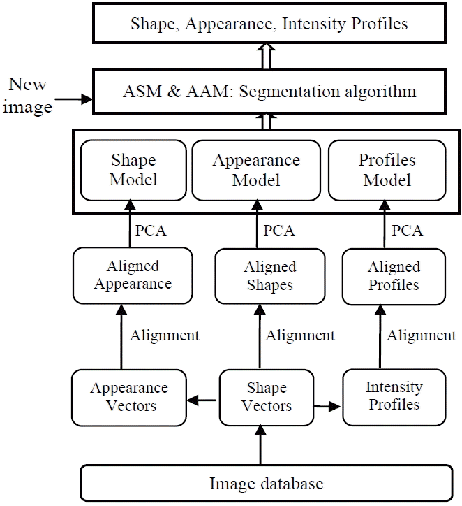
Fig. 2
(a) Landmarks and a normal vector direction at a specific landmark point, (b) the intensity profile, and (c) the gradient profile. 
Fig. 3
Global schema of parallel AAM (Active Appearance Model) model. 
Fig. 4
Data parallel model (f is the same function). 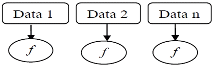
Fig. 5
(a) Landmarks and a normal vector direction at a specific landmark point j, (b) the intensity profile [ 24]. 
Fig. 6
(Top) an example of a simple shape with four points. (Down) the same shape as a vector [ 16]. 
Fig. 7
Method for calculation of profile’s gradient [ 16]. 
Fig. 8

Fig. 9
Parallel method of local appearance model of an image [ 16]. 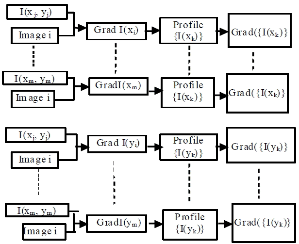
Fig. 10
(a) Summary of Principal Component Analysis (PCA) and (b) PCA transformation. 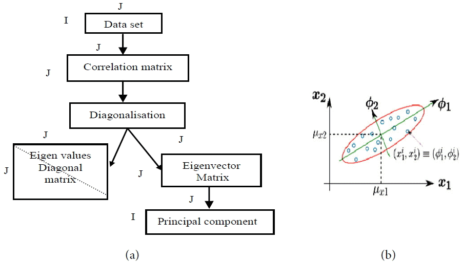
Fig. 11
(a) Shape space and (b) variable space. 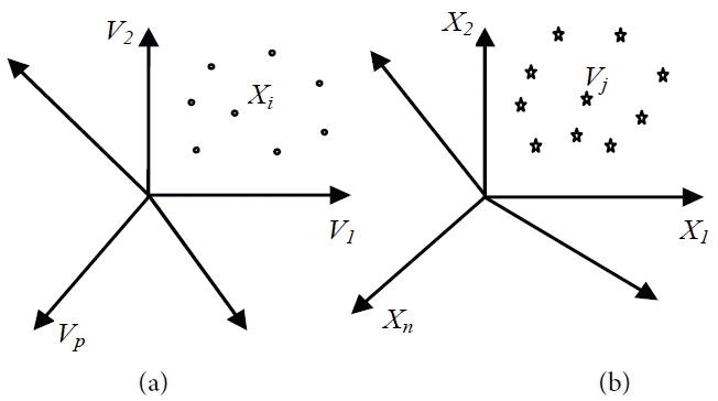
Fig. 12
Two principal components analyzes for abscissa and ordinate separately. 
Fig. 13
Distributed scheme for parallel model of Active Appearance Model. 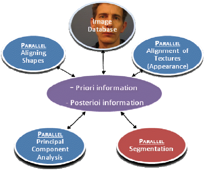
Fig. 14
(a) Distributed schema and parallel of profile procedure and (b) distributed schema and parallel of alignment procedure. 
Fig. 15
Distributed Schema and parallel of PCA. 
Fig. 16
(a) The annotated mouth using 8 landmarks for images of JAFFE (Japanese Female Facial Expression) database, (b) interfaces of the calculation of intensity profiles. 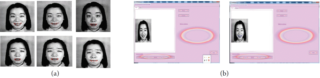
Fig. 17
(a) Annotated mouth, (b) image gradient in X, (c) image gradient in Y, and (d) plotting of intensity profiles. 
Fig. 18
(a) PCA intefaces and (b) mean shapes. 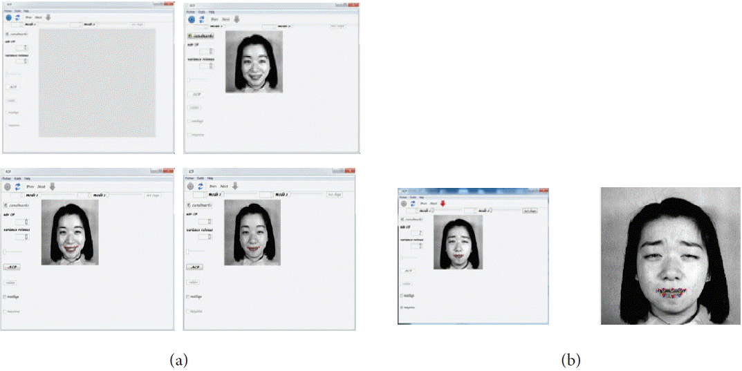
Fig. 19
(a) PCA application execution and (b) results obtained and execution times. 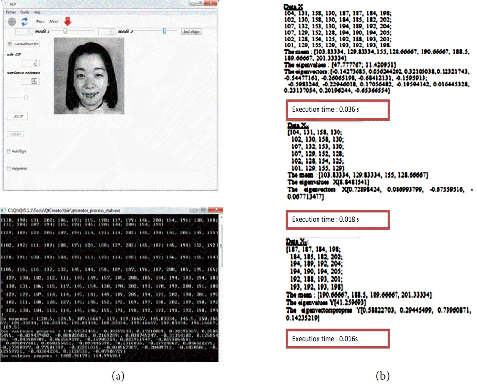
|


