A Chi-Square-Based Decision for Real-Time Malware Detection Using PE-File Features
Article information
Abstract
The real-time detection of malware remains an open issue, since most of the existing approaches for malware categorization focus on improving the accuracy rather than the detection time. Therefore, finding a proper balance between these two characteristics is very important, especially for such sensitive systems. In this paper, we present a fast portable executable (PE) malware detection system, which is based on the analysis of the set of Application Programming Interfaces (APIs) called by a program and some technical PE features (TPFs). We used an efficient feature selection method, which first selects the most relevant APIs and TPFs using the chi-square (KHI2) measure, and then the Phi (ϕ) coefficient was used to classify the features in different subsets, based on their relevance. We evaluated our method using different classifiers trained on different combinations of feature subsets. We obtained very satisfying results with more than 98% accuracy. Our system is adequate for real-time detection since it is able to categorize a file (Malware or Benign) in 0.09 seconds.
1. Introduction
Computer systems are a real asset for organizations and corporations in today’s technology-driven economy. Unfortunately, they are confronted with several kinds of cyber attacks. Among the most used attacks are those based on installing and running a malware in target machines. Malware (e.g., Trojans, viruses, worms, etc.) are computer programs, which are designed to accomplish unauthorized actions without the user’s consent. Malware can be used to steal or damage data or to disrupt network traffic. Moreover, the compromised machines can be used as “zombies” in order to conduct targeted attacks, such as DDOS [1]. Recently, we are witnessing an unprecedented and a very concerning proliferation of malware. McAfee has reported that more than 30 million new malware were discovered during the first quarter of 2014; that number was double the amount for the the same period of 2013 [2,3]. This malicious software infects thousands of computers every day, and Microsoft Windows operating system (OS) remains the most affected, as it is the most used OS worldwide. During January 2015, about 80% of computers ran on MS Windows OS [4]. Under the latter operating system, malware are often present as legitimate executable files, and they can have any known file extension (e.g., exe, com, etc.). Therefore, they are structured according to a common executable file format called PE (portable executable) [5] (see Section 2).
Efficiently protecting computers against malware attacks has become vital for companies, corporations, and individuals. Unfortunately, the existing commercial antivirus (AV) software is unable to provide the required level of protection. Techniques used by most AVs are signature-based. A signature is a short and unique string of bytes, which is recorded in the signature’s database for each known malware so that future examples of it can be correctly classified with a small error rate. Such techniques suffer from two major drawbacks: First, they need to have a prior knowledge of malware by their signatures. Therefore, they are unable to detect unknown or newly launched (zero-day) ones [6,7]. Second, they are inefficient against metamorphic malware (i.e., variants of known malware) [6,8]. Recently, AV software has become more effective by using more sophisticated analysis techniques. However, there is still the problem of delay, which can vary from a few hours to several days, between the detection of a new malware and the updating of the viral databases by the AV firms [7,9,10]. During this period, the malware could cause considerable damages.
In the last decade, researchers employed more sophisticated malware detection methods, such as behavioral and heuristic analyses [11,12], as an alternative to signature-based ones. Behavioral analysis, which is also known as dynamic analysis, consists of observing the behavior of a program at runtime, by monitoring its execution in an isolated environment (Sandbox or virtual machine). During the monitoring process, the actions that the program accomplishes (such as library uses, kernel calls, network traffic, and registry updates) are recorded and used to generate features for classifying the program (malware or benign). The main advantage of dynamic analysis is that it can detect unknown and metamorphic malware [10]. However, new evasive methods that can detect the analysis environment and completely stop the execution of the malware code or delay the execution of its malicious content until the monitoring process is terminated have been introduced. Note that the monitoring process is run for a couple of minutes at most, which itself is inconvenient since it cannot observe the entire capabilities of a given program as not all execution paths can be explored [10]. Furthermore, such techniques are not suitable for real-time purposes.
On the other hand, heuristic-based analysis uses data mining and machine learning techniques to learn the behavior of the program [11]. Such techniques investigate different file features, such as Opcode instructions, structural information, and APIs. These sets of information are represented in different forms (e.g., control flow graphs, n-grams, etc.) and are used as features for the classification process, which is generally done using different classifiers, such as decision trees and Bayes algorithm. API calls were widely used for constructing anti-malware systems [6,8,10,13–16], since they can provide valuable information related to the possible behaviors that a given program could have [16]. Indeed, the operating system provides APIs to user applications allowing them to request its services. Also, some authors [12] have investigated structural information due to its robustness against code obfuscation techniques, such as packing.
The heuristic-based anti-malware systems are able to detect unknown and metamorphic malware [11,17]. They are also easy to implement compared to the behavioral ones. However, heuristic-based systems suffer from the inconvenience of their high false positive rate (i.e., benign programs that are wrongly detected as malware) [11]. In order to overcome this drawback, most of the existing systems combine a large number of different types of features [11]. This can lead to intensive computations and increase the processing time. Due to that, most of the actual heuristic-based anti-malware systems are inadequate for real-time detection, which is a suitable characteristic, especially in a dynamic environment (i.e., a malware analysis environment). Therefore, being able to find an appropriate balance between accuracy and detection time is a real challenge when constructing anti-malware systems.
In this work, we introduce an efficient heuristic-based PE-malware detection system, which has a real-time response and a low false alarm rate. The proposed system is composed of a feature extraction module, a pre-processing module, a feature selection module, and a decision module. The feature extraction module statically (i.e., without running the program) extracts the set of API calls from the Import Address Table (IAT), and the technical PE features (TPF) from the PE-optional header (see Section 2). The feature selection module is based on the KHI2 test, which is a statistical method used for hypothesis testing [18]. We introduce the Phi (ϕ) measure for feature set reduction, which means that the decision will be taken according to the most significant features. The latter allows for a real-time response. The decision module is based on different data mining based classifiers that have been implemented in the Waikato Environment for Knowledge Analysis (WEKA) [19]. For experimentation purposes, we used two sets of files — a benign set and a malware set — that we obtained from well-known dedicated databases. To the best of our knowledge, our work is the first to use a combination of the KHI2 measure and the ϕ coefficient as a feature reduction method and to use this combination with a hybridization of features (APIs + TPFs).
This paper is organized as follows: in Section 2, we introduce the PE file format and its structure, in order to facilitate comprehension about the rest of the sections. Section 3 is devoted to the best-known related works, published in the literature. In Section 4, we present the proposed malware detection system, and in Section 5 we present our experimental results. In Section 6, we introduce our analysis of the obtained results, and we compare the performance of our system with the existing ones. Section 7 concludes our work and underlines its perspectives.
2. PE File Format
PE is the common file format for binary executables and DLLs in Windows OS. A PE file is mainly composed of an MS-DOS header, PE header, and Section headers (section table), and a set of sections [5], as shown in Fig. 1.

Simplified PE-file structure.
The MS-DOS header is located at the beginning of the PE-file and it is used to check whether it is a valid executable or not, when the file is run under DOS.
The PE-header contains some important pieces of information about the PE-file. The PE-header is an IMAGE_NT_HEADERS data structure that contains three members, which are signature, file header, and the optional header (Fig. 2).
The PE-optional headerisan IMAGE_OPTIONAL_HEADER structure, and it is composed of several fields, such as Magic, MajorLinkerVersion, and CheckSum [5]. One of the PE-optional header fields is the data directory, which is an array of 16 IMAGE_DATA_DIRECTORY structures. One of these structures is the IMAGE_DIRECTORY_ENTRY_IMPORT, which contains information about all the imports (DLLs/APIs). The import entry points to a vector of IMAGE_IMPORT_DESCRIPTOR structures. The field “OriginalFirstThunk” of the latter structure contains an RVA (Relative Virtual Address), which points to the IAT, as shown in Fig. 2. The IAT is an array of function pointers that contains elements of IMAGE_THUNK_DATA structures. Each structure corresponds to an imported API, and they contain the ordinal of a function or an RVA to an IMAGE_IMPORT_BY_NAME structure. The latter contains the names of the APIs that the code calls.
Structure of the PE-optional header and location of the IAT.
3. Related Works
In this section, we provide a brief description of some often-cited works in the literature that have used APIs, PE features, or a KHI2-based decision to detect malware files.
Schultz et al. [16] introduced the first anti-malware system based on machine learning techniques. They investigated different information in the PE file, such as strings, API functions, and byte sequence. They used a classification method based on the naïve Bayes algorithm, and they obtained an overall accuracy of 97.11%. The method introduced in [13] uses naïve Bayes classification with API calls. The extracted APIs were used to construct models of suspicious behaviors, by grouping some APIs based on scenarios that a malware can accomplish, such as searching for a file to infect and writing malicious data into it. They obtained 93.7% accuracy.
Ye et al. [6] proposed CIMDS, which is an improvement of their previous malware detection system called IMDS (Intelligent Malware Detection System) [8]. As its predecessor, CIMDS is based on Object Oriented Association (OOA) mining. They used the KHI2 method for rule pruning (removing insignificant rules), rule ranking (from most significant to least significant), and rule selection (best nAPIs). CIMDS was the first work that used post-processing techniques. The system achieved 67.5% accuracy and 88.16% detection rate, which still needs improvements. However, it has a very good detection time with 0.09 seconds per file. The authors in [14] also presented a malware detection system based on OOA mining and API calls. They proposed a feature selection method to reduce the number of obtained APIs by selecting the top 1,000 ones based on two criteria, which are document frequency and information gain. The system achieved 91.2% accuracy and a detection rate of 97.3%.
The authors in [17] combined the KHI2 test and the hidden Markov model (HMM) for detecting malware using an Opcode sequence. They extracted Opcode from the analyzed files using the third party disassembler IDA Pro. They used the KHI2 test to identify the set of instructions that are most likely to be used by the NGVCK malware generator to generate malware variants. They then learned the HMM using the set of obtained instructions in order to categorize the files. They tested their method on 200 malware and 40 benign programs. Their proposed system had an overall accuracy of 91%. The drawback of this method is the usage of a closed source disassembler (IDA Pro), which makes their system not fully automatic. Moreover, their analysis was limited to malware that is generated using NGVCK.
The method described in [15], extracts API calls and compares them to previously constructed models of malicious APIs stored in a signature’s database. A similarity measure between the extracted model and the existing one was calculated by combining three different metrics, which are cosine similarity, extended Jaccard measure, and Pearson correlation. After that, they selected the most relevant features using a weighting scheme. The weight of an API was obtained by calculating the product of two metrics, which are term frequency and inversed document frequency. The classification phase was based on a Support Vector Machine (SVM) classifier and they obtained an overall accuracy of 91.5%.
The authors in [10] proposed a malware detection system that is based on analyzing API functions and their arguments. They used a dynamic feature extraction method using a virtual environment. They evaluated their method using different classifiers, and they obtained an overall accuracy of 98.1%. Using arguments requires program being executed. Consequently, this method suffers from the inconveniences of dynamic approaches, which were previously mentioned.
PE-Miner [12] was introduced as a real-time framework for PE-malware detection. This framework statically extracts PE-files structural features from the PE header, optional header, etc. The authors proposed a method based on information gain to select the most relevant features. They evaluated their framework using five different data mining classifiers. The proposed framework was able to achieve a detection rate of more than 99% and a false alarm rate of about 5%. The categorization process takes an average of 0.244 seconds per file.
4. Proposed System
Our proposed method for PE-malware categorization is based on the observation that there are some PE-file features that are specific to malware and others to benign programs. These features appear with different frequencies between these two categories of PE-files. Therefore, these features must be extracted and sorted in a way that we consider to be only the most significant ones that will make a significant contribution in the benign-malware categorization process. Thus, the statistical KHI2 test is used to estimate the significance (relevance) of these features. Thus, we will provide, at the same time, a real-time detection of PE-malware and a high specific categorization using small sets of features.
4.1 System Architecture
Our proposed system for malware detection is composed of four different modules, which are the feature extraction module, pre-processing module, feature selection module, and the decision module, as shown in Fig. 3.

4.2 Feature Extraction
As mentioned previously, our system relies on the analysis of two different types of features, which are API calls and some TPFs. The TPFs are represented by the information stored in the PE-optional header fields. In order to extract these two types of features from a PE file and calculate their frequencies, we developed a module written in Python that uses a third-party Python module called Pefile, which is a multi-platform module for reading and working with PE files and extracting different information from them [20]. This extraction method is based on a static analysis of the IAT for API calls and the PE-optional header for the TPFs (see Section 2). Given below in Figs. 4 and 5, is an overview of some lines of Python code that we wrote to extract API calls and TPFs from multiple PE files contained in a folder named “Malware_Samples.”

Python source code for extracting API calls (for API in entry.imports) and storing them in APIs structure (API_LIST).
Python source code for extracting TPFs (pe.OPTIONAL_HEADER…) and storing them in TPFs structure (TPF_LIST).
Note that TPFs are represented by concatenating the field’s name with its value (e.g., ‘checksum0’), as shown in lines 8 and 9 of the above source code (Fig. 5).
4.3 Pre-processing
After extracting APIs and TPFs using the previous module, the pre-processing module proceeds in removing duplicated APIs in the same PE file, and then it calculates their call frequencies in malware and benign files. The module also calculates the frequency of appearances of the obtained TPFs in malware and benign programs. At the end of this phase we obtained a table composed of three columns that, respectively, represent the feature’s name, its frequency in malware PE, and its frequency in benign PE, and a number of rows, which is equal to the number of obtained features (APIs + TPFs) (see Subsection 5.2).
4.4 Feature Selection
The third module of our system is the feature selection module. It was also developed as a Python script, and it aims at selecting the most relevant features from the obtained list of APIs and TPFs. This module is based on a well-known statistical method, which is the KHI2 hypothesis test [18]. This method is used to decide whether there is a significant association between two qualitative variables. This association is expressed by the distance D between an observed frequency O and an expected one E, which represents the case of perfect independence between the variables). Therefore, the correlation strength between two variables is proportional to the distance D. In our case, we studied the association between two variables: First, the variable “Feature” that has two modalities of “present” and “not present.” This variable represents the presence or absence of a feature (API or TPF) in a PE file. Second, the variable “PE-cat,” which also has the two modalities of “malware” and “benign.” This variable represents the two categories of PE files, for instance: “malware” and “benign.” When conducting a KHI2 test, we first started by defining the two hypotheses H0 and H1, where one will be accepted and the other rejected. H0 (null hypothesis) represents the case of independence between the two variables. H1 (alternative hypothesis) represents the case of dependency between the two variables. In our case, H0 and H1 are defined as follows:
H0 : The presence or absence of a feature (API, TPF) is independent of the PE file’s type (malware or benign).
H1 : The presence or absence of a feature (API, TPF) is related to the PE file’s type (malware or benign).
For each feature F, we had a contingency table, as shown in Table 1.

Contingency table of a feature F
We describe below the different variables presented in Table 1.
M and N are, respectively, the total number of malware and benign PE files.
T is the total number of used PE files (T=M+N).
M1 is the number of malware PE files that contain F, and M2 is the number of malware PE files that do not contain F, such as M=M1+M2.
N1 is the number of benign PE files that contain F, and N2 is the number of benign PE files that do not contain F, such as N= N1+N2.
Based on the contingency table (Table 1), the KHI2 score (D2) is calculated using Eq. (1).
where, Or,c is the observed frequency count at level r of the row variable and level c of the column variable. And Er,c is the expected frequency, which is defined by the following equation :
where, nr and nc are, respectively, the sum of row r and the sum of column c. After calculating the KHI2 values for the extracted features, we had to determine which of the two hypotheses H0 or H1 would be accepted or rejected for every feature. To do that, we compared the obtained KHI2 values (D2) of every feature to a threshold, which represents the theoretical KHI2 value (χ2), and H0 was accepted (H1 rejected) for every feature that had D2≤ χ2. Note that according to the KHI2 hypothesis test, the features for which H0 is accepted are considered to be irrelevant and will be systematically removed. The χ2 value is obtained by first calculating the degree of freedom (DF), and choosing a signification level α that represents the probability of rejecting a hypothesis even if is true. Considering DF and α, the χ2 value is obtained from the KHI2 distribution table [21]. DF is calculated as follows:
where R and C represent, respectively, the number of modalities of the first and the second variables. After removing all the features that are not correlated, which correspond to the case where H0 is accepted, we calculated the ϕ coefficient for the remaining features. The ϕ coefficient [22] is a normalization of the KHI2 score (D2), which can only be applied to a 2×2 contingency tables (two variables with two modalities). It is used to measure the strength of the dependency between the two variables [23]. In our work, this coefficient was used to group features in subsets according to their correlation strength (relevance). ϕ is calculated as follows:
The value of ϕ ranges between 0 and 1, and the relevance of a feature (API or TPF) is proportional to that value. Therefore, we chose to use three subsets that would contain features that have ϕ≥0.25, ϕ≥0.5, and ϕ≥0.75, respectively. Our aim was to be able to identify the optimal number of features required to have the highest accuracy, which also helps to reduce the detection time.
4.5 Decision
After generating the different features’ subsets from the previous module, we had to identify which of the APIs or TPFs or combinations of them provided the best results (i.e., high accuracy and low detection time). Therefore, we first evaluated our system using TPFs subsets. We then used APIs subsets, and, finally, we evaluated it by trying every possible combination of the TPFs-APIs subsets. We used different classification algorithms available in WEKA, which are the decision tree (J48) [19], boosted decision tree (B-J48) using the AdaBoostM1 algorithm [19], Rotation Forest (Rot-F) [24], and Random Forest (Ran-F) [25]. Our decision module took the features’ subsets generated from the feature selection module and the set of extracted ones from the analyzed file as input. Both are represented as WEKA data files (.arff file) [19], which are automatically generated using a Python script.
5. Experimentation
5.1 Dataset
For experimentation purposes, we collected a dataset composed of 552 PE files (338 malware and 214 benign programs), of 80% were used as the training set and 20% as the test set. The infected PE files were downloaded from Vxheavens.com and contained 12 different malware categories, as shown in Table 2.
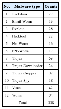
Malware dataset
The benign PE files include some utility software that was downloaded from Softpedia.com, and also some Windows system files that were collected from a clean installation of Windows XP. In our work, we only considered non-packed (non-compressed) programs. Packing is a method that is legitimately used by software developers to protect their programs from reverse engineering, and malware creators use it to hide the malicious code from being detected by AV software [26]. Therefore, we analyzed our dataset using well-known Packers detection tools, such as PEiD, and ProtectionID. These tools are able to detect a large variety of packers, including popular ones like UPX, ASPack, and PECompact. Note that packed binaries are the only category that was excluded from our samples. We also scanned all the files using more than 40 different AVs from the website VirusTotal.com. More than 30 AVs identified the infected PE files that were used as malware, and none of the benign PE files were identified as malware.
5.2 Results
In this subsection, we present the results obtained from the feature extraction phase to the decision phase. After the feature extraction and pre-processing phases, we obtained the results presented in Tables 3 and 4.
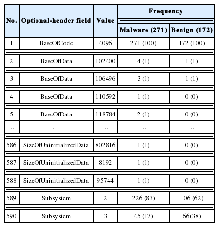
Overview of the obtained TPFs

Overview of the obtained APIs
We calculated the KHI2 values for the obtained APIs and TPFs and removed the irrelevant ones that had KHI2 ≤ 3.84 (3.84 is the χ2 value for DF=1 and alpha=0.05). Thus, H0 was rejected and H1 was accepted for 681 APIs and 50 TPFs, and H0 was accepted and H1 was rejected for 959 APIs and 540 TPFs. The results are presented in Tables 5 and 6.
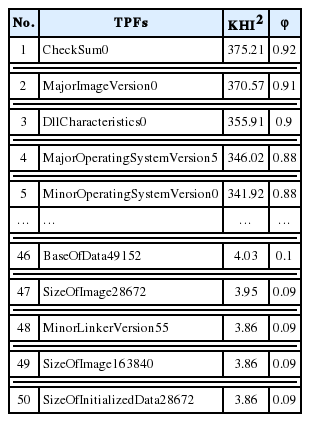
Overview of the obtained KHI2 and ϕ values for the selected TPFs
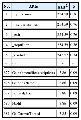
Overview of the obtained KHI2 and ϕ values for the selected APIs
As mentioned previously, we obtained a final list of 681 APIs and 50 TPFs with their corresponding KHI2 scores and ϕ values, as shown in Tables 5 and 6. We divided these features into different groups (subsets) according to their ϕ values. At the end of the feature selection phase, we obtained three subsets for APIs, which are A1, A2, and A3, and three subsets for TPFs, which are H1, H2, and H3. The latter subsets correspond, respectively, to the three ϕ values, which are ϕ≥0.75, ϕ≥0.5, and ϕ≥0.25. We obtained 5, 31, and 297 APIs in A1, A2, and A3, respectively. We also obtained 11, 14, and 22 TPFs in H1, H2, and H3. We used a fourth subset for both APIs (A4) and TPFs (H4) that contained all of the extracted features (1,640 APIs and 590 TPFs). The purposed of using these two additional subsets was to see whether the proposed feature selection method improved our system’s performance or not.
In the next subsection, we evaluate our system’s performance by using different classifiers with the obtained features’ subsets and see which subset or combination of subsets generates the best results.
5.3 Evaluation
Our experiments were conducted on a Windows 7 OS, I3-2350M 2.30 GHZ CPU, and 4GB of RAM computer. The feature extraction, pre-processing, and selection modules were implemented in Python 27. The decision module was implemented in WEKA 3.7.
The performance of a malware detection system is generally evaluated according to three different metrics, as discussed below.
-
Detection rate (DR): This represents the percentage of malware detected among all malware of the given test set, and it is calculated using Eq. (5):
(5) -
False alarm rate (FA): This is the percentage of benign files wrongly classified as malware among all the benign files of the given test set, and it is calculated using Eq. (6):
(6) -
Accuracy (AC): This represents the rate of files that were correctly classified in their class, and it is calculated using Eq. (7):
(7)
Since we want to achieve a real-time detection of malware, we must take into consideration the detection time (DT) as a fourth metric to evaluate our system’s performance. DT represents the average time required for categorizing a given PE file from our test set, and it is expressed in seconds per file. The obtained results are presented in Tables 7–9.

Experimental results using TPFs subsets

Experimental results using APIs subsets

Experimental results (best classifier) using combinations of API-TPF subsets
We can see from the results presented in the table above that our system has the highest AC with the subset H2 (97.25%), with an improvement of 1.84% compared with the obtained AC using the subset H4 (no feature selection). In addition, the average detection time was also reduced (−0.004s).
The results presented in Table 8 show that our system is more accurate with the subset A2 and Rot-F classifier. Compared with the subset A4 there was an improvement of 1.27%. The detection time was reduced by 40% from 0.136s (A4+Ran-F) to 0.081s (A2+Rot-F). By comparing the results in Table 7 and Table 8, we can see that TPFs provided a better accuracy (97.28%) compared with APIs (96.20%), and a better detection time (−0.004s). Next, we combined both APIs and TPFs in order to increase accuracy. The results are presented in Table 9 and include only the best classifier scores.
As can be seen from the obtained results, we were able to improve the accuracy of our system, compared with TPFs only (+0.67%) and APIs only (+1.84%), and that by combining H2 and A3 subsets using B-J48. Furthermore, we were able to keep a good detection time with an average of 0.090 s. We were also able to achieve the same accuracy with the combination of H3 and A3 subsets using the same classifier, but with a detection time of 0.092 s. Therefore, we prefer to consider the first combination (H2+A3). From the results previously presented, we can conclude that the proposed feature selection method made a very important contribution in increasing the system’s accuracy and in reducing the detection time.
6. Comparison and Discussion
In this section, we evaluate the efficiency of our system by comparing our obtained results to those of the previously cited systems, as presented in Table 10 and Fig. 6.
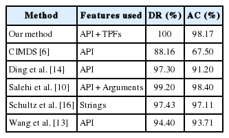
Comparison of our results with previously cited methods having used the same evaluation metrics
Histogram comparing our system’s AC and DR with those of the previously cited ones.
From the results presented in the above table, is can be seen that our system outperforms four of the five presented systems in terms of accuracy, with an improvement that varies from 1.06% to 30.67%. The method proposed by Salehi et al. [10] had a better accuracy than our method with an improvement rate of 0.23%. However, our system has the best detection rate compared to all of these systems.
Considering the detection time (categorization time), we can conclude that our system is adequate for the real-time detection of malware, since it only requires 0.090s for the whole categorization process. Our system has the same detection time as CIMDS [6], and it is almost three times faster than PE-Miner [12], as the latter takes 0.244s to categorize a file.
Our proposed feature extraction and pre-processing method took 0.040s, 0.037s, and 0.041s for APIs, TPFs, and APIs + TPFs, respectively. These results are very satisfying compared with the method used in [10], which needs to monitor the analyzed program for two minutes in order to extract the API calls and their arguments, which is almost 3,000 times the amount of time required for our proposed method.
The time cost for generating the .arff file depends on the number of features used. For instance, it took 0.037s with A1+H1, 0.049s with H3+A3, and 0.142s for H4+A4. Note that the arff file generation process is related to the usage of the WEKA environment. Therefore, its time cost was not taken into consideration when the classifier was directly implemented and integrated in our system.
The time cost for the classification process depends on the number of used features and the classification method. For instance, with H1+A1 subsets and the B-J48 classifier, the classification process took 0.001s, with H2+A3 using the same classifier it took 0.004s, and using the Rot-F classifier it took 0.119s.
7. Conclusion and Future Works
In this work, we have presented a fast PE-malware detection system that is based on the analysis of API calls and TPFs. The KHI2 test was used as the feature selection method and was combined with the ϕ coefficient, which was used to select the optimal number of features. Different classification algorithms were used to evaluate our system. The results show that our system is more accurate when the APIs and TPFs are combined using a B-J48 classifier, as we achieved an overall accuracy of 98.27%. Our system is automatic and can be used for the real-time detection of malware. As for future work, we will try to increase the accuracy of our system by combining other types of features and at the same time, we will try to keep the same rapidity. We also intend to study the different API associations that are specific to the different malware categories, which will allow for the multiclass categorization of malware.
References
Biography
Mohamed Belaoued http://orcid.org/0000-0002-9412-1959

He received his B.A. and M.A. degrees both in computer science from the University of Skikda, Algeria in 2009 and 2011, respectively. He is now and since 2011 a PhD student within the department of computer science of the same university. His main research interests include computer security, distributed systems, and data mining.
Smaine Mazouzi

He is an associate professor at 20 Août 1955 University of Skikda. He received his M.S. and Ph.D. degrees in Computer Science from University of Constantine, respectively, in 1996 and 2008. His fields of interest are pattern recognition, machine vision, and computer security. His current research concerns using distributed and complex systems modeled as multi-agent systems in image understanding and intrusion detection.