A New Image Clustering Method Based on the Fuzzy Harmony Search Algorithm and Fourier Transform
Article information
Abstract
In the conventional clustering algorithms, an object could be assigned to only one group. However, this is sometimes not the case in reality, there are cases where the data do not belong to one group. As against, the fuzzy clustering takes into consideration the degree of fuzzy membership of each pixel relative to different classes. In order to overcome some shortcoming with traditional clustering methods, such as slow convergence and their sensitivity to initialization values, we have used the Harmony Search algorithm. It is based on the population metaheuristic algorithm, imitating the musical improvisation process. The major thrust of this algorithm lies in its ability to integrate the key components of population-based methods and local search-based methods in a simple optimization model. We propose in this paper a new unsupervised clustering method called the Fuzzy Harmony Search-Fourier Transform (FHS-FT). It is based on hybridization fuzzy clustering and the harmony search algorithm to increase its exploitation process and to further improve the generated solution, while the Fourier transform to increase the size of the image’s data. The results show that the proposed method is able to provide viable solutions as compared to previous work.
1. Introduction
The processing of any image can be seen as a semi-structured data and complex. The extraction of information offers new opportunities and challenges for the researchers. Several image-processing techniques have been developed to correctly and efficiently use the quality of information, including clustering, which was developed in the 1960s. Whether supervised or not, the objective is to extract the maximum information that exists in an image by identifying the various classes that constitute the depicted scene that it is feasible to get a comprehensible and interpretable form. The supervised methods require a user’s description of the classes, while the unsupervised ones are independent from the user [1].
Several metaheuristic algorithms that have been described in the literature were used for classification: genetic algorithms, particle swarm optimization, support vector machines, etc., and this area has seen the emergence of a new generation of algorithm-inspired systems and biological phenomena. The Harmony Search (HS) algorithm is one of these techniques. The HS is a metaheuristic optimization algorithm developed by Geem et al. [2] in 2001. It has a soft computing technique that is similar to the genetic algorithm [3], and it has the capacity to exploit the new solution proposed (harmony) with the synchronization of the search space where intensification and diversification of environmental optimization are parallel [4]. The HS algorithm was inspired by the observation that the purpose of a musician is to produce a piece of music with perfect harmony, which is analogous to finding the optimality in an optimization process. Research process optimization can be compared to the jazz improvisation process. On the one hand, the perfect harmony pleasant is determined by aesthetic estimation [5,6].
The effectiveness and benefit of the HS algorithm has been demonstrated in various applications. It has been applied to solve many optimization problems in civil, mechanical, and electrical engineering as an efficient optimization algorithm that often finds a solution faster than genetic algorithms or neural network algorithms [7,8]. It has also proved to be very successful in many other diverse fields, including computer vision, image segmentation, vehicle routing, and music composition [3,9]. The principal advantages of the HS optimization algorithm are summarized as follows [10,11]: 1) HS imposes fewer mathematical requirements; 2) HS does not require complex calculus, thus it is free from divergence; 3) HS uses stochastic random searches, thus any derivative information is unnecessary; 4) HS creates a new solution vector after considering all of the existing solution vectors; 5) HS does not require initial value settings for the decision variables, thus it may escape local optima; and 6) HS can easily handle discrete variables and continuous variables.
The purpose of this study is to investigate the HS algorithm and design a new approach to improve the performance of clustering in an image-processing problem. Clustering or unsupervised classification in an image can indeed be obtained using a clustering applied to a set of pixel values (e.g., grayscale, color, or spectral responses). To increase the size of the downloaded image’s data, the Fourier transform is applied and then a hybridization of the HS algorithm and fuzzy clustering is performed for solving the classification task [1]. We then demonstrate the effectiveness of our clustering approach in different type of images (synthetic, artificial, photographic, and satellite).
The rest of the paper is organized as follows: Section 2 presents the basic fundamental of fuzzy clustering. In Section 3, we explain the Fourier transform and we describe in Section 4 the HS metaheuristic algorithm in detail. Section 5 is devoted to the Fuzzy Harmony Search-Fourier Transform (FHS-FT) clustering algorithm. Implementation and results are discussed in Section 6 and the conclusion and future work are presented in Section 7.
2. Fuzzy Clustering
As has been previously defined, a clustering algorithm is typically performed on a set of n patterns or objects X={x1, x2,…, xn}, where each xi ε Rd is a feature vector consisting of d real-valued measurements describing the features of the object represented by xi [12] and its objective consists of assigning the elements to only one group.
Two types of clustering algorithms are available: hard and fuzzy. In hard clustering, the goal is to partition the dataset X into non-overlapping, non-empty partitions G1,…, Gc, whereas, in fuzzy clustering algorithms the goal is to partition the dataset X into partitions that allow the data object to belong in a certain (possibly null) degree to every fuzzy cluster [12].
However, in reality, there are situations where the data does not belong to only one group, and these situations cannot be solved by exact clustering. Contrary to fuzzy clustering, the vectors can belong to more than one group. A membership value indicates the degree of membership of an element in each group [13,14]. Consider the following example:
This example (Fig. 1) shows the case of partitioning a set of objects according to their shapes and colors. We see that in the case of the red and blue squares has been the exception partitioning. This situation illustrates the imprecision and uncertainty related to the membership of the object to more than one group. The solution to this problem lies in the introduction of fuzzy logic, by adding a membership value that indicates the degree of membership of an element with different groups [12–14].
Imprecision and uncertainty partitioning.
This implies that the clustering output is a membership matrix called a fuzzy partition matrix U = [uij]c x n, as shown in Eq. (1), where, uij ∈ [0, 1] indicates the membership of the ith element to the jth group of the fuzzy cluster. The fuzzy partitioning of the data follows the following conditions:
Where, c is the cluster, n is data of the image (pixel), and uij represents the membership degree of a pixel i in group j, and cj is the center of the group j, we have:
As well as fuzzy clustering, there are several validity indices to evaluate the quality of fuzzy partitioning. We included the Jm index and XB index [12,15], which are two of the best-known indices.
3. Fourier Transform
A rectangular matrix whose elements correspond to the color value of each pixel represents a digital image. In the case of black and white images (2D signals), this value is the light intensity of the pixels in the space and in the case of sound (1D signals), this value is then amplitude changes sound over time [16,17]. This type of easy transformation creates many advantages regarding image processing.
The notion of the Fourier transform of the 2D signals is a generalization of the 1D signals. The Fourier transform of the image allows for the switching of representation in the spatial or temporal domains to representation in the frequency domain [17]. In the case of images (2D signals), the lower frequencies are large homogeneous areas and blurred parts, while the high frequencies represent contours (abrupt intensity changes) and noise [16].
3.1 Mathematically
For 2D signals (images), we defined their Fourier transform by the following mathematical formula:
Let f(x,y) be a function of two variables representing the intensity of an image, with:
X,Y as the spatial coordinates
vx,vy as the spectral coordinates.
We see from the expression of the FT that F(vx,vy) is generally a complex number, even if f(x,y) is a real number. Thus, F(vx,vy) has amplitude and a phase. One can choose to represent either one or the other, and we were only interested that the amplitude [16,17]. And reciprocally the inverse Fourier transform is as follows:
This transformation is reversible and can be written as:
Nevertheless, in computer science, all of the signals used are sampled and quantized. Therefore, only the discrete equivalent (DFT) of the continuous Fourier transform is used. The mathematical definition of a signal s for N samples is as follows:
The inverse transform is given by:
3.2 Adjustment
The frequencies are arranged unnaturally on the resulting image, as shown below:
It is considered much more natural to have low frequencies in the center of the image and high ones in the periphery (Fig. 2). As such, we chose to interchange the quadrants. Doing so did not change the result, because the image of the transform is periodic and the DFT can be made in any part of image Typically the low frequencies in the images are much more present (broad and slow intensity variations); thus, the majority of the content is in the center of the frequency spectrum [16].
Result of the Fourier transform and after inversion of the quadrants (left to right).
3.3 Filtering and Convolution
The convolution product is related to the concept of filtering. A filter is linear and time invariant (time independent). The Fourier transform of the convolution product of two functions is simply the product (classical) of their Fourier transform and reciprocally [16,17].
As such, we were able to use a spatial or frequency filter in an equivalent way. The latter option only involves multiplication, which makes it less expensive.
For interpretation of the Fourier transform in terms of high and low frequencies, if we implemented the following variable change on FT: (u, v) → (ω, θ), then the value of F(ωcosθ, ωsinθ) for a pair (ω, θ) gives the amplitude of a sinusoid complex in pulsation ω in the direction θ (Fig. 3).
Low frequencies and high frequencies in the Fourier plane.
For many images, the middle (in terms of probabilities) of the amplitude is independent of the direction θ and decreases steadily with ω. If we decrease the amplitude of the high frequency (low-pass filtering according to ω for all values of θ), the image appears blurred and the edges are less sharp. If instead, we increase the amplitude at high frequencies, the contours are enhanced, but the image seems noisier (it has a larger grain) [17].
Thus, we concluded that for high frequency filtering that far from the center frequency of the FT is the opposite for Bas frequency filtering, and for the frequency near the center of FT and a band frequency filtering (average) we created a band circle between the high and low frequency.
4. Harmony Search Algorithm
The HS algorithm is a metaheuristic algorithm that was developed by Geem et al. [2] in 2001 for optimization problems. It mimics the process of the musicians playing their instruments and attempting to create a well-balanced harmony. It has a soft computing technique that is similar to the genetic algorithm [3] and it has the capacity to exploit our proposed solution vector (harmony vector) with the synchronization of the search space where intensification and diversification environmental optimization are parallel [4].
The HS algorithm takes several solution vectors into consideration simultaneously, and this procedure is similar to the genetic algorithm. However, the major difference between the genetic algorithm and the HS algorithm is in the reproduction process. While the HS algorithm generates a new vector from all of the existing vectors, the genetic algorithm generates a new vector from only two parents. In addition, iterations in the HS algorithm are faster than in the genetic algorithm [18,19].
To explain the research of harmony in greater detail, we must understand the process of improvisation by a skilled musician. Each musician remembers the good pitches in order to replay them again with the hopes of generating a fantastic harmony in their next practice session [20].
As such, each musician has three possible choices to improvise a pitch from his/her instrument [6,10,20], which are as follows:
Playing any famous pitch exactly from his/her memory.
Playing a pitch similar to a memorized pitch.
Composing a new pitch from a possible range of pitches.
The improvisation process of a musician in finding a New Harmony follows the following three rules [1,2,20]:
Harmony Memory Consideration (HMC): A decision value is picked from a stored solution in the Harmony Memory (HM) with the probability of the Harmony Memory Consideration Rate (HMCR).
Pitch Adjustment (PA): Decides whether the chosen decision value from the HM can be adjusted to the neighboring values with a probability of HMCR × Pitch Adjustment Rate (PAR).
Random Search (RS): A decision value picked randomly from a defined range with a probability of (1-HMCR).
Optimization algorithms seek the best state (i.e., global optimum), which is determined by the objective function value. As such, for the HS algorithm, musical performances search for a perfect state of harmony, which is determined by aesthetic estimation. The pitch of each musical instrument determines the aesthetic quality; just as the objective function value is determined by the set of values assigned to each design variable.
The solution procedure of the HS algorithm is controlled using three parameters [4,21]: HMS, HMCR, and PAR. These parameters are defined in the following section. The solution of an optimization problem using the HS algorithm (shown in Fig. 4) is performed based on following five steps [20,22–24]:
Optimization procedure of the improved harmony search algorithm.
Step 1. Initialize the optimization problem and HS algorithm parameters. Initialize the parameter of the HS algorithm, the number of decision variables, values range, HMS (i.e., the number of vectors in the solution of harmony memory), HMCR where HMCR ∈ [0, 1], PAR where PAR ∈ [0, 1], and the stopping criteria (i.e., the number of iterations [IT]).
Step 2. Initialize the harmony memory. Initialize the HM by generating solution vectors from the decision variable (the entire search space of the problem to be optimized).
Step 3. Improvise a New Harmony. Improvise a new solution vector using HM, HMCR, PAR, RS, and the three HS algorithm improvisation rules.
Step 4. Update the harmony memory. If the new improvised solution vector is better than the worst solution vector in the HM, replace the worst solution with the new improvisation (in terms of the objective function value).
Step 5. Check the stopping criterion. Check for convergence. If convergence or stopping criteria have not been met go back to Step 3, otherwise take out the best solution in the HM as the optimal solution vector of the function.
5. Clustering by Fuzzy Harmony Search–Fourier Transform
The FHS-FT algorithm is a hybrid method between the HS algorithm, fuzzy logic, and Fourier transform. In this section, we describe the FHS-FT algorithm, and also show how it addresses the problem of image clustering.
Table 1 presents the analogy of the FHS-FT clustering algorithm with a musician’s improvisation process in regards to finding a New Harmony and optimization problem:
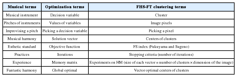
FHS-FT clustering vs. musical terms and optimization terms
5.1 Image Representation
Clustering is applied on a set of artificial images, photographic images, and satellite’s images. For the satellite image, LANDSAT5 Thematic Mapper (TM), our algorithm began by loading the three images corresponding to the three channels TM2, TM3, and TM4. After this we did a color composition by associating the blue filter with channel TM2, the green filter with channel TM3, and the red filter with channel TM4. As such, we used 3D RGB images.
5.2 Fourier Transform Application
The purpose of using the Fourier transform in this work is to identify the frequency characteristics of an image. We focused only on the Fourier spectrum (i.e., the modulus of the Fourier transform) of the image, without worrying about the phase. Indeed, the spectrum can account for the energy distribution of the image, and with respect to the periodicity that of the orientation of the image patterns, this is especially convenient in the study of the image.
This phase consists of loading three images corresponding to the dimension of the images, but for satellite images it corresponds to the TM2, TM3, and TM4 channels. Then, we performed the Fourier transform and frequency filters (low pass, band pass and high pass) for each image. As a result, we had 12 images to load in our algorithm, the three dimensions of images, and the images after applying frequency filters.
5.3 Initialization of Parameters
Initializing the values of the FHS-FT algorithm’s parameters is very important for obtaining the best optimization results because these parameters can seriously affect the performance of the algorithm.
For the maximum number of classes in the image, we estimated the number of classes constituting, in a visual way, the image, and we fixed a random value greater than it. However, the choice of parameters values related to FHS-FT: HMS, HMCR, PAR and IT (iterations number) were selected from our previous studies made with the HS algorithm and which are presented in articles [5,25,26] where the recommended range for the number of generations or iterations (IT) were between 50 and 200 (for an artificial image) and between 200 and 2,000 (for a satellite image), the size of harmony memory (HMS) was 20, the HMCR between 0.7 and 0.9, and the PAR between 0.1 and 0.5. However, the best value of HMCR and PAR that produced the best optimal results presented in our articles [5,25,26] were 0.9 and 0.1, respectively.
5.4 Initialization of Harmony Memory
The HM matrix in Eq. (8) is initialized with randomly generated solution vectors as many as the HMS = 20 (the possible range of decision variables ak of solution vectors is between 0 to 255.) with their respective values of the objective function [4,24], as explained in Section 5.5.
Each vector harmony memory (HM vector) is a solution of the cluster centers of the FHS-FT algorithm, which has a physical length of (c × d) [4], where, c is the number of clusters and d is the dimension of the image. The vector of the solution is as shown in Eq. (9):
For example, if an image has three different regions, that is 3D (RVG) three characteristics that describe each pixel, the harmony vector could be as (120, 52, 80, 50, 150, 20, 196, 240, and 33), wherein (120, 52, and 80) represent the value centers of the cluster for the first image region, and (50, 150, and 20) represent the value centers of the cluster for the second image region, and so on.
5.5 FHS-FT Process
After loading the satellite image RGB, application TF, initialization of the FHS-FT parameters, and the HM, the FHS-FT algorithm starts working, and for each iteration, a New Harmony vector (solution vector) x’=(x1’, x2’,⋯, xcxd’) is generated by considering three rules of improvising a New Harmony (memory consideration, pitch adjustment, and random) until the stopping criterion is reached, as shown in Fig. 4.
In regards to memory consideration, it is possible to choose the value of the decision variable from the y values stored in the HM range x’=(x11, x12,⋯, xcxdHMS ) [24]. It uses the HMCR parameter, which varies between 0 and 1, and is the probability of selecting one value from HM; whereas (1-HMCR), is the probability of randomly selecting from the possible range. The selection procedure for HMCR is shown in Eq. (10) [10,19]:
The HMCR is the probability of choosing one value from the historic values stored in the HM, and (1- HMCR) is the probability of randomly choosing one possible value that is not limited to those stored in the HM. For example, an HMCR of 0.95 indicates that the FHS-FT algorithm will choose the design variable value from previously stored values in the HM with a 95% probability rate and from the entire feasible range with a 5% probability rate. A HMCR value of 1.0 is not recommended because of the possibility that the solution may be improved by values not stored in the HM. This is similar to the reason why the genetic algorithm uses a mutation rate in the selection process [27].
After the memory is taken into consideration, each decision variable choice is evaluated to determine whether pitch adjustment is necessary or not [24]. This procedure uses the PAR parameter, which is identified in Eq. (11). It sets the rate of adjustment for the pitch chosen from the HM as shown in Fig. 5.
New Harmony improvisation concept.
The parameter PAR means “changing the frequency” of the simulated music. This means that the PAR generates slightly different values for the composition of the New Harmony vector and explores more additional solutions in the search space.
Here, bw is a bandwidth distance that is arbitrarily used to improve the performance of the HS, and in this paper it is set to bw = 0,0001 MaxValeur (n); where MaxValeur (n) = 255 is the maximum value that can take a pixel and rand () is a uniform random number between 0 and 1.
As can be seen in Eq. (11), the decision variable xi’ is replaced with xi’ ← xi’ ± rand (0,1) × bw with probability PAR, while doing nothing with probability (1-PAR) [10,13,19].
Through this process, the fitness value of each new vector will be calculated and compared with the worst fitness value in harmony memory [4,28].
If the new vector’s fitness value is better or equal than that worst value in HM, replacement will take place and this new vector will be as a new vector in the HM; otherwise, it will be ignored. Once the HS algorithm has met the stopping criterion, the selection of a solution vector with minimum fitness value is made in HM to reach its goal of finding the optimal cluster centers.
5.6 Objective Function
The objective function or validity index is utilized to calculate the fitness of the solution. The FHS-FT algorithm is based on optimizing an objective function and it’s FS index. According to our previous studies, which are presented in [5], the FS validity index increases the performance of the algorithm for satellite image clustering compared to the Jm, XB, and DB validity indices [1,5,13,15].
The FS index in Eq. (12), was proposed by Fukuyama and Sugeno in 1989. Where, m=1, xk is the kth data point, vi are cluster prototypes (cluster centers), c is the number of clusters, v is the grand mean of all data xk, uik is the membership value of data xk of class ci, and |ci| is the total amount of data belonging to cluster i.
6. Experimental Results and Analysis
For comparing the performance of the FHS-FT algorithm, which we have proposed for the clustering of optical data, we studied different type of images (artificial, photographic, and satellite). In this section, we describe the images used, the parameters of the algorithm FHS-FT, experiences, results, and discussions.
6.1 Image Used
The experiments conducted were applied on five different images (two synthetics, one artificial, one photographic, and one satellite) to better evaluate our proposed algorithm. The first and second images are synthetics that contain three and five clusters or colors, respectively (Fig. 6). The third image is artificial and contains three clusters, and the fourth image is a photograph of vegetables that contains four clusters (Fig. 6). The last image is a satellite image provided by QUICKBIRD. The natural disaster that we chose to detect was an earthquake, which was 6.8 [29] on the Richter scale, in the Boumerdes region (in Algeria) dated May 21, 2003 (Fig. 7).
Images used (image 1, 2, 3 and 4 from left to right).
Satellite image used and study area.
The satellite image shown in Fig. 7 is in high resolutions and is a colorful composition of the three channels (LANDSAT 5 TM bands in 4, 3, and 2 RGB). We used just a part of the LANDSAT 5 TM (Thematic Mapper) seismic satellite image (Area A in Fig. 7) and it contains five different clusters (area damage, asphalt, soil, vegetation, and shadows).
6.2 Experiences and Discussion
The objective of these experiments that we conducted was to measure quality and analyze the optimized performance of our FHS-FT algorithm for clustering or the unsupervised classification of different types of images.
For our first test, we applied four experiments to image 1 (Fig. 6), which contains three clusters (red, blue, and yellow). The first experience was with the HS classic algorithm proposed in [25], the second was with the HS algorithm that works with the FS validity index proposed in [5,26,29], the third with FHS algorithm proposed in [30], and the last experience with our new FHS-FT algorithm. While we fixed the same parameters for the four algorithms according to Section 5.1, the number of clusters or classes had a random value of more than three, 1 iteration number (IT=1), and other parameters of HMS=20, HMCR=0.9, and PAR=0.1. The results obtained from the experiences applied to image 1 are summarized in Table 2.
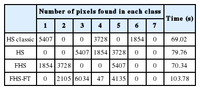
Results of the clustering on image 1 by the four algorithms
Table 2 shows that the classes constituting image 1 were correctly recognized depending on the number of clusters detected (equal to 3) in the HS classic, HS, FHS, and FHS-FT algorithms. There was only a small difference in the run time, so the HS classic algorithm is better because it considers the index Jm as the membership value of data of class uij, while the HS used the index Fs, the FHS algorithm used the index Fs with consideration the membership of data of class uij (fuzzy logic), and the FHS-FT algorithm used the index Fs, fuzzy logic, and the Fourier transform.
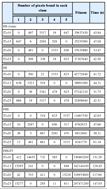
For the second test on image 2 (Fig. 6), which contained five clusters (colors red, blue, green, yellow, and purple), we kept the same parameters formed in image 1 (HMS=20, HMCR=0.9, PAR=0.1) and only changed the parameter IT from 10 to 40. For the number of clusters, the random value was more than five. All of these experiences were carried out with the HS classic, HS, FHS, and FHS-FT algorithms. The different results obtained about the fitness, the number of clusters recognized, and the run time of each algorithm, are summarized in the Tables 3 and 4 below. The experiences, which are shown in Table 4, were the best results obtained for each iteration of each algorithm (i.e., for every iteration we conducted several tests and kept the best). They were chosen depending on the minimum fitness and visual recognition rates of image classification.
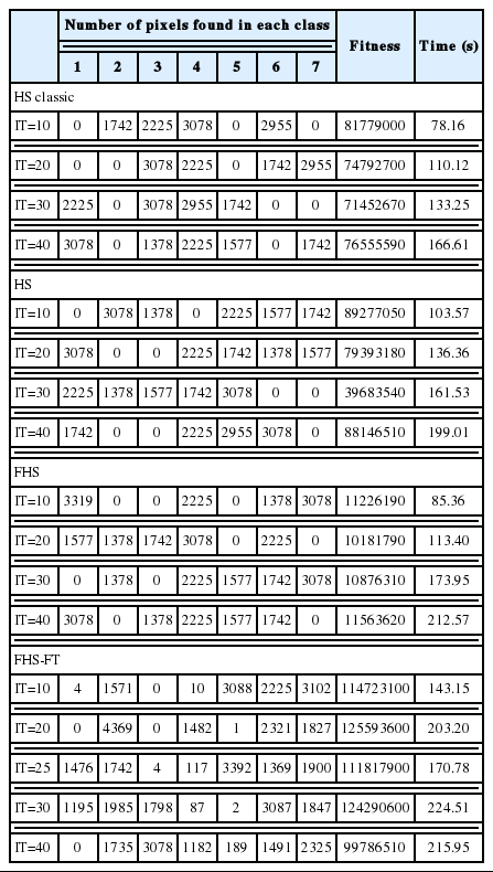
Results of the clustering on image 2 by the four algorithms
Results by image of the clustering on image 2 by the four algorithms
Depending on the basis of the results for the unsupervised classification of image 2, which are shown in Tables 3 and 4, we observed that the best result obtained for the HS classic algorithm was in the number of iterations equal to 40, for the HS algorithm it was in the number of iterations equal to 30, for the FHS algorithm it was in the number of iterations equal to 20, and for the FHS-FT algorithm it was is in the number of iterations equal to 40. These results are based on the minimum fitness rate and number of classes recognized equal to 5 (visual recognition rate). When the number of iterations and the run time of the best results between the algorithms were compared, the FHS algorithm was the best because it provides a better performance for clustering a synthetic image compared the other algorithms in terms of clustering, the number of iterations, and execution time.
For the third test on image 3 (Fig. 6), we kept the same parameters (HMS=20, HMCR=0.9, PAR=0.1) and algorithms as before. In these tests, we used an artificial image that contained three clusters (red, white, and black), so the number of clusters had a random value of more than three, and the parameter IT varied from 10 to 25. The results obtained from experiences used in image 3 are summarized in Tables 5 and 6. The experiences shown in Table 5 are the best results obtained for each iteration.
Results of the clustering on image 3 by the four algorithms
Results by image of the clustering on image 3 by the four algorithms
From the results obtained in Tables 5 and 6 about the supervised classification of an artificial image (image 3 in Fig. 6) by the four algorithms, we noted that the best result was given by the FHS algorithm where the number of iterations was 10. This is because the number of classes recognized was equivalent to 3 as compared to other iteration tests (IT=15, 20, and 25). The other best algorithm results for the HS classic algorithm it was 20 iterations, for the HS algorithm it was 13 iterations, and for the FHS-FT algorithm it was 13 iterations.
Once again, the FHS algorithm is the best, because it provides better performance for clustering a synthetic image compared the other algorithms in regards to clustering, the number of iterations, and execution time.
From these tests, shown in Tables 3 and 5, it can be noted that the variation of the number of iterations influxes in regards to results in two different ways: the more we increased the number of generations, we had a better clustering; but arrive at a number of generations, the performance of our algorithm began to degrade. We concluded that the determination of the IT is very sensitive, because it can lead to divergence. The latter is caused by the operation rand (0, 1), which consists of incorporating the modifications of the harmony solution vector at each iteration and initial memory.
Results of the clustering on image 4 by the four algorithms
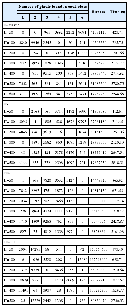
In the fourth test, we used a photographic image (image 4 in Fig. 6) that contained four clusters (red and green for the peppers, white and black for light) and the number of clusters had a random value of more than four. In regards to experiences, the parameters of the four algorithms were like the preceding experiences (HMS=20, HMCR=0.9, PAR=0.1); but just for the IT parameter, we varied it from 50 to 600. The results, which are summarized in Tables 7 and 8, are the best results obtained for each iteration, and they were chosen depending on the minimum fitness and visual recognition rates of image classification.
Results by image of the clustering on image 4 by the four algorithms
According to the results given in Tables 7 and 8 for photographic image clustering (image 4 in Fig. 6), the algorithm that gave the best visual recognition rate was the FHS-FT with an IT equal to 400. This was because the classified image was the closest to the real image, even if in iterations equal to 500 is the best fitness value and equal to 200 is the best number of the recognized classes (equal to 4). However, despite the increased recognition rate (visual) in 400 iterations, there were minimal upgrades compared to other algorithms. The results were as follows: green class: blue 3937 pixels and green 63 pixels; white class: yellow 1373 pixels and pink 8 pixels; and the red and black classes: red 11491 pixels and orange 28 pixels. Some confusion persisted, primarily in the black and red classes, because our algorithm found that they are of the same class.
For the other algorithms the results were as follows: the HS classic algorithm had a 600 IT, the HS algorithm had a 400 IT, and the FHS algorithm had a 400 IT. When we compared the best FHS-FT result with other algorithms, we saw that the upgrade rates (of FHS, HS, and HS classic) were more than the FHS-FT algorithm. For example, in the FHS algorithm an orange upgrade (762 pixels) in white and black classes; in HS algorithm an upgrade with color blue (424 pixels) and red (48 pixels) in white class, and also a confusion between white and green class; in HS classic algorithm an upgrade in color green (609 pixels) in red class and color orange (587 pixels) in black class, and also a confusion between classes: white with green, black with green and red. We concluded that the FHS-FT algorithm is the best because it provides better performance for clustering a photographic image compared to other algorithms in regards to the visual recognition rate of the clustering, the number of iterations, the execution time, and upgrade.
For the last test, we used a satellite image (Area 1 in Fig. 7). Our experiment consisted of extracting the information that we desired to obtain from a satellite image by using unsupervised classification (clustering), because classification is an important step in the processing phase. The purpose of processing is obtaining the visual interpretation of the image processed for analysis, understanding the target, and helping to solve the issue of the management of natural disasters (detection of natural disasters). As we have presented in Section 6.1, we used part of a LANDSAT5 TM satellite image seismic area (earthquake in the Boumerdes region dated May 21, 2003), and it contained five different clusters (area damage, asphalt, soil, vegetation, and shadows). For this experience we used the same algorithms and parameters (HMS=20, HMCR=0.9, PAR=0.1) as we did for the others. The number of clusters had a random value of more than five and the parameter IT varied from 10 to 100. The best results obtained for each algorithm (i.e., for every iteration we ran several tests and kept the best results, which were chosen based on the minimum fitness and visual recognition rates of image classification) are summarized in Table 9.
Results by image of the clustering on image 5 by the four algorithms
From Table 9, which contains the results of the satellite image clustering by the four algorithms, we can conclude that if we compare the results with the actual image area (because we know this area), the quality of the clustering using the FHS-FT algorithm provides a very good rate of visual recognition of area damage (light blue 9890 pixels). Also, according to the results obtained with the other algorithms it is more precise, but there is a little confusion between asphalt and soil classes (like the other algorithms). There is also a small upgrade in soil class (green 7340 pixels and pink 32 pixels) and in asphalt class (orange 6907 pixels and blue 182 pixels).
However, it is important to note that the FHS-FT causes fewer false alarms and little confusion in regards to the asphalt and soil classes (green, orange) and the upgrade in soil class (green, pink) compared to the others algorithms.
So, from the experiments, which are shown in Tables 2–9, the FHS-FT algorithm has a good performance in clustering and fewer false alarms (good detection of area damage and other classes) of the satellite and photographic images, as compared to FHS, HS, and HS classic. However, it has a weakness in clustering simple statics images. The FHS algorithm gives the best result because these types of images do not need to apply the FT since they are not complex pictures.
7. Conclusions and Future Work
Classification is always the key point in the field of image processing. The fuzzy clustering model is an essential tool for finding the proper cluster structure of given data sets in pattern and image classification. However, this algorithm usually has some weaknesses, such as the problem of falling into a local minimum, and it needs a lot of time to accomplish the classification for a large amount of data. In order to overcome these shortcomings and increase classification accuracy, we hybridized the HS algorithm with the Fourier transform (FT) to obtain an improved algorithm (FHS-FT) for unsupervised classification.
The experimental results on benchmark images (photographic and satellite) show that the FHS-FT algorithm presents a novel concept that imports significant improvements to complex image clustering, and is more promising for the recognition of real world objects in unknown scenes.
For the future work, we propose including an initialization method in our FHS-FT approach and to extend this method by using the texture parameter in the classification process in order to increase the accuracy of identifying the areas of natural disasters.
References
Biography
Ibtissem Bekkouche
She received License and Master degree in Computer Science from the University of Science and Technology of Oran ‘Mohamed Boudiaf’ in 2008 and 2010, respectively. Since January 2010, she is with the Faculty of Computer Science from University of Mohamed Boudiaf as a PhD candidate. Her research interests include: image processing, classification algorithms development for remotely sensed data and analysis of spatial data.
Hadria Fizazi
She is currently a Professor in the Faculty of Computer Science in the University of Science and Technology of Oran ‘Mohamed Boudiaf’. Engineer degree in Electrical Engineering from the University of Mohamed Boudiaf in 1981, the “doctor Engineer” degree in Industrial Computer Science and Automation from the University of Lille 1 France in 1987 and the Doctorate degree in Computer Science from the University of Mohamed Boudiaf in 2005. Her research interests cover image processing and the application of pattern recognition to remotely sensed data.